Classification with KerasHub
- 원본 링크 : https://keras.io/guides/keras_hub/classification_with_keras_hub/
- 최종 확인 : 2024-11-19
저자 : Gowtham Paimagam, lukewood
생성일 : 09/24/2024
최종 편집일 : 10/22/2024
설명 : Use KerasHub to train powerful image classifiers.
Classification is the process of predicting a categorical label for a given input image. While classification is a relatively straightforward computer vision task, modern approaches still are built of several complex components. Luckily, Keras provides APIs to construct commonly used components.
This guide demonstrates KerasHub’s modular approach to solving image classification problems at three levels of complexity:
- Inference with a pretrained classifier
- Fine-tuning a pretrained backbone
- Training a image classifier from scratch
KerasHub uses Keras 3 to work with any of TensorFlow, PyTorch or Jax. In the guide below, we will use the jax backend. This guide runs in TensorFlow or PyTorch backends with zero changes, simply update the KERAS_BACKEND below.
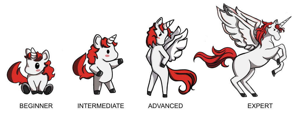
We use Professor Keras, the official Keras mascot, as a visual reference for the complexity of the material:
!!pip install -q --upgrade keras-hub
!!pip install -q --upgrade keras  # Upgrade to Keras 3.
import os
os.environ["KERAS_BACKEND"] = "jax" # @param ["tensorflow", "jax", "torch"]
import json
import math
import numpy as np
import matplotlib.pyplot as plt
import keras
from keras import losses
from keras import ops
from keras import optimizers
from keras.optimizers import schedules
from keras import metrics
from keras.applications.imagenet_utils import decode_predictions
import keras_hub
# Import tensorflow for [`tf.data`](https://www.tensorflow.org/api_docs/python/tf/data) and its preprocessing functions
import tensorflow as tf
import tensorflow_datasets as tfds결과
['',
 '\x1b[1m[\x1b[0m\x1b[34;49mnotice\x1b[0m\x1b[1;39;49m]\x1b[0m\x1b[39;49m A new release of pip is available: \x1b[0m\x1b[31;49m23.0.1\x1b[0m\x1b[39;49m -> \x1b[0m\x1b[32;49m24.2\x1b[0m',
 '\x1b[1m[\x1b[0m\x1b[34;49mnotice\x1b[0m\x1b[1;39;49m]\x1b[0m\x1b[39;49m To update, run: \x1b[0m\x1b[32;49mpip install --upgrade pip\x1b[0m']
Inference with a pretrained classifier

Let’s get started with the simplest KerasHub API: a pretrained classifier. In this example, we will construct a classifier that was pretrained on the ImageNet dataset. We’ll use this model to solve the age old “Cat or Dog” problem.
The highest level module in KerasHub is a task. A task is a keras.Model consisting of a (generally pretrained) backbone model and task-specific layers. Here’s an example using keras_hub.models.ImageClassifier with an ResNet Backbone.
ResNet is a great starting model when constructing an image classification pipeline. This architecture manages to achieve high accuracy, while using a compact parameter count. If a ResNet is not powerful enough for the task you are hoping to solve, be sure to check out KerasHub’s other available Backbones!
classifier = keras_hub.models.ImageClassifier.from_preset("resnet_v2_50_imagenet")You may notice a small deviation from the old keras.applications API; where you would construct the class with Resnet50V2(weights="imagenet"). While the old API was great for classification, it did not scale effectively to other use cases that required complex architectures, like object detection and semantic segmentation.
We first create a utility function for plotting images throughout this tutorial:
def plot_image_gallery(images, titles=None, num_cols=3, figsize=(6, 12)):
    num_images = len(images)
    images = np.asarray(images) / 255.0
    images = np.minimum(np.maximum(images, 0.0), 1.0)
    num_rows = (num_images + num_cols - 1) // num_cols
    fig, axes = plt.subplots(num_rows, num_cols, figsize=figsize, squeeze=False)
    axes = axes.flatten()  # Flatten in case the axes is a 2D array

    for i, ax in enumerate(axes):
        if i < num_images:
            # Plot the image
            ax.imshow(images[i])
            ax.axis("off")  # Remove axis
            if titles and len(titles) > i:
                ax.set_title(titles[i], fontsize=12)
        else:
            # Turn off the axis for any empty subplot
            ax.axis("off")

    plt.show()
    plt.close()
Now that our classifier is built, let’s apply it to this cute cat picture!
filepath = keras.utils.get_file(
    origin="https://upload.wikimedia.org/wikipedia/commons/thumb/4/49/5hR96puA_VA.jpg/1024px-5hR96puA_VA.jpg"
)
image = keras.utils.load_img(filepath)
image = np.array([image])
plot_image_gallery(image, num_cols=1, figsize=(3, 3))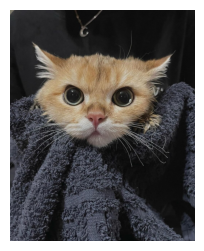
Next, let’s get some predictions from our classifier:
predictions = classifier.predict(image)결과
1/1 ━━━━━━━━━━━━━━━━━━━━ 0s 12s/step


1/1 ━━━━━━━━━━━━━━━━━━━━ 12s 12s/step
Predictions come in the form of softmax-ed category rankings. We can use Keras’ imagenet_utils.decode_predictions function to map them to class names:
print(f"Top two classes are:\n{decode_predictions(predictions, top=2)}")결과
Downloading data from https://storage.googleapis.com/download.tensorflow.org/data/imagenet_class_index.json
0/35363 [37m━━━━━━━━━━━━━━━━━━━━ 0s 0s/step
35363/35363 ━━━━━━━━━━━━━━━━━━━━ 0s 0us/step
Top two classes are:
[[('n02123394', 'Persian_cat', -1.3963771), ('n02808304', 'bath_towel', -2.0231562)]]Great! Both of these appear to be correct! However, one of the classes is “Bath towel”. We’re trying to classify Cats VS Dogs. We don’t care about the towel!
Ideally, we’d have a classifier that only performs computation to determine if an image is a cat or a dog, and has all of its resources dedicated to this task. This can be solved by fine tuning our own classifier.
Fine tuning a pretrained classifier

When labeled images specific to our task are available, fine-tuning a custom classifier can improve performance. If we want to train a Cats vs Dogs Classifier, using explicitly labeled Cat vs Dog data should perform better than the generic classifier! For many tasks, no relevant pretrained model will be available (e.g., categorizing images specific to your application).
First, let’s get started by loading some data:
BATCH_SIZE = 32
IMAGE_SIZE = (224, 224)
AUTOTUNE = tf.data.AUTOTUNE
tfds.disable_progress_bar()

data, dataset_info = tfds.load("cats_vs_dogs", with_info=True, as_supervised=True)
train_steps_per_epoch = dataset_info.splits["train"].num_examples // BATCH_SIZE
train_dataset = data["train"]

num_classes = dataset_info.features["label"].num_classes

resizing = keras.layers.Resizing(
    IMAGE_SIZE[0], IMAGE_SIZE[1], crop_to_aspect_ratio=True
)


def preprocess_inputs(image, label):
    image = tf.cast(image, tf.float32)
    # Staticly resize images as we only iterate the dataset once.
    return resizing(image), tf.one_hot(label, num_classes)


# Shuffle the dataset to increase diversity of batches.
# 10*BATCH_SIZE follows the assumption that bigger machines can handle bigger
# shuffle buffers.
train_dataset = train_dataset.shuffle(
    10 * BATCH_SIZE, reshuffle_each_iteration=True
).map(preprocess_inputs, num_parallel_calls=AUTOTUNE)
train_dataset = train_dataset.batch(BATCH_SIZE)

images = next(iter(train_dataset.take(1)))[0]
plot_image_gallery(images)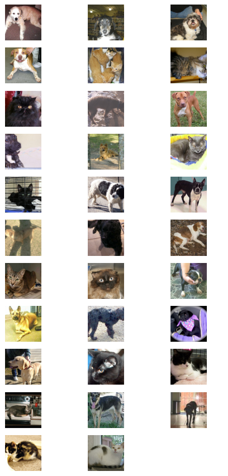
Meow!
Next let’s construct our model. The use of imagenet in the preset name indicates that the backbone was pretrained on the ImageNet dataset. Pretrained backbones extract more information from our labeled examples by leveraging patterns extracted from potentially much larger datasets.
Next lets put together our classifier:
model = keras_hub.models.ImageClassifier.from_preset(
    "resnet_v2_50_imagenet", num_classes=2
)
model.compile(
    loss="categorical_crossentropy",
    optimizer=keras.optimizers.SGD(learning_rate=0.01),
    metrics=["accuracy"],
)
Here our classifier is just a simple keras.Sequential. All that is left to do is call model.fit():
model.fit(train_dataset)결과
1/727 [37m━━━━━━━━━━━━━━━━━━━━ 4:54:54 24s/step - accuracy: 0.5312 - loss: 4.9475 2/727 [37m━━━━━━━━━━━━━━━━━━━━ 2:59 247ms/step - accuracy: 0.5469 - loss: 4.9475
3/727 [37m━━━━━━━━━━━━━━━━━━━━ 2:51 236ms/step - accuracy: 0.5660 - loss: 4.9475
727/727 ━━━━━━━━━━━━━━━━━━━━ 219s 268ms/step - accuracy: 0.6553 - loss: 0.7275
<keras.src.callbacks.history.History at 0x7f5b2888e670>Let’s look at how our model performs after the fine tuning:
predictions = model.predict(image)

classes = {0: "cat", 1: "dog"}
print("Top class is:", classes[predictions[0].argmax()])
결과
1/1 ━━━━━━━━━━━━━━━━━━━━ 0s 2s/step


1/1 ━━━━━━━━━━━━━━━━━━━━ 2s 2s/step

Top class is: cat
Awesome - looks like the model correctly classified the image.
Train a Classifier from Scratch

Now that we’ve gotten our hands dirty with classification, let’s take on one last task: training a classification model from scratch! A standard benchmark for image classification is the ImageNet dataset, however due to licensing constraints we will use the CalTech 101 image classification dataset in this tutorial. While we use the simpler CalTech 101 dataset in this guide, the same training template may be used on ImageNet to achieve near state-of-the-art scores.
Let’s start out by tackling data loading:
BATCH_SIZE = 32
NUM_CLASSES = 101
IMAGE_SIZE = (224, 224)

# Change epochs to 100~ to fully train.
EPOCHS = 1


def package_inputs(image, label):
    return {"images": image, "labels": tf.one_hot(label, NUM_CLASSES)}


train_ds, eval_ds = tfds.load(
    "caltech101", split=["train", "test"], as_supervised="true"
)
train_ds = train_ds.map(package_inputs, num_parallel_calls=tf.data.AUTOTUNE)
eval_ds = eval_ds.map(package_inputs, num_parallel_calls=tf.data.AUTOTUNE)

train_ds = train_ds.shuffle(BATCH_SIZE * 16)
augmenters = []
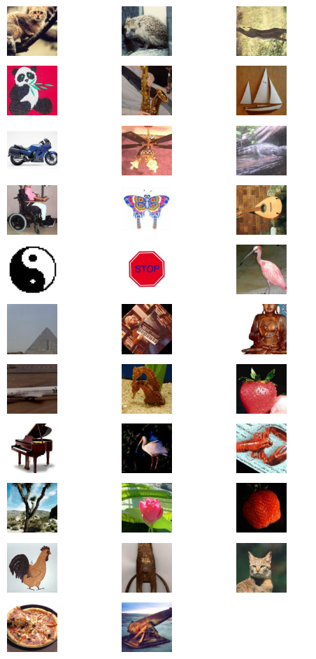
The CalTech101 dataset has different sizes for every image, so we resize images before batching them using the batch() API.
resize = keras.layers.Resizing(*IMAGE_SIZE, crop_to_aspect_ratio=True)
train_ds = train_ds.map(resize)
eval_ds = eval_ds.map(resize)

train_ds = train_ds.batch(BATCH_SIZE)
eval_ds = eval_ds.batch(BATCH_SIZE)

batch = next(iter(train_ds.take(1)))
image_batch = batch["images"]
label_batch = batch["labels"]

plot_image_gallery(
    image_batch,
)
Data Augmentation
In our previous finetuning example, we performed a static resizing operation and did not utilize any image augmentation. This is because a single pass over the training set was sufficient to achieve decent results. When training to solve a more difficult task, you’ll want to include data augmentation in your data pipeline.
Data augmentation is a technique to make your model robust to changes in input data such as lighting, cropping, and orientation. Keras includes some of the most useful augmentations in the keras.layers API. Creating an optimal pipeline of augmentations is an art, but in this section of the guide we’ll offer some tips on best practices for classification.
One caveat to be aware of with image data augmentation is that you must be careful to not shift your augmented data distribution too far from the original data distribution. The goal is to prevent overfitting and increase generalization, but samples that lie completely out of the data distribution simply add noise to the training process.
The first augmentation we’ll use is RandomFlip. This augmentation behaves more or less how you’d expect: it either flips the image or not. While this augmentation is useful in CalTech101 and ImageNet, it should be noted that it should not be used on tasks where the data distribution is not vertical mirror invariant. An example of a dataset where this occurs is MNIST hand written digits. Flipping a 6 over the vertical axis will make the digit appear more like a 7 than a 6, but the label will still show a 6.
random_flip = keras.layers.RandomFlip()
augmenters += [random_flip]

image_batch = random_flip(image_batch)
plot_image_gallery(image_batch)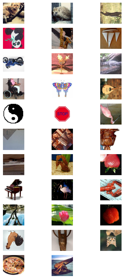
Half of the images have been flipped!
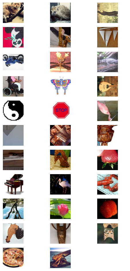
The next augmentation we’ll use is RandomCrop. This operation selects a random subset of the image. By using this augmentation, we force our classifier to become spatially invariant.
Let’s add a RandomCrop to our set of augmentations:
crop = keras.layers.RandomCrop(
    int(IMAGE_SIZE[0] * 0.9),
    int(IMAGE_SIZE[1] * 0.9),
)

augmenters += [crop]

image_batch = crop(image_batch)
plot_image_gallery(
    image_batch,
)
We can also rotate images by a random angle using Keras’ RandomRotation layer. Let’s apply a rotation by a randomly selected angle in the interval -45°…45°:
rotate = keras.layers.RandomRotation((-45 / 360, 45 / 360))

augmenters += [rotate]

image_batch = rotate(image_batch)
plot_image_gallery(image_batch)

resize = keras.layers.Resizing(*IMAGE_SIZE, crop_to_aspect_ratio=True)
augmenters += [resize]

image_batch = resize(image_batch)
plot_image_gallery(image_batch)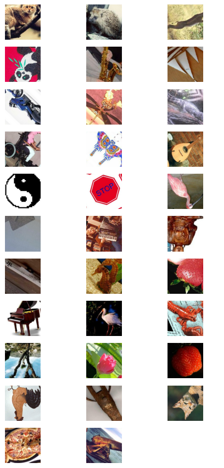

Now let’s apply our final augmenter to the training data:
def create_augmenter_fn(augmenters):
    def augmenter_fn(inputs):
        for augmenter in augmenters:
            inputs["images"] = augmenter(inputs["images"])
        return inputs

    return augmenter_fn


augmenter_fn = create_augmenter_fn(augmenters)
train_ds = train_ds.map(augmenter_fn, num_parallel_calls=tf.data.AUTOTUNE)

image_batch = next(iter(train_ds.take(1)))["images"]
plot_image_gallery(
    image_batch,
)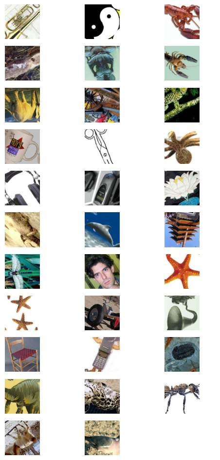
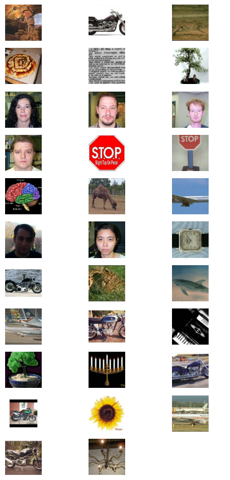
We also need to resize our evaluation set to get dense batches of the image size expected by our model. We directly use the deterministic keras.layers.Resizing in this case to avoid adding noise to our evaluation metric due to applying random augmentations.
inference_resizing = keras.layers.Resizing(*IMAGE_SIZE, crop_to_aspect_ratio=True)


def do_resize(inputs):
    inputs["images"] = inference_resizing(inputs["images"])
    return inputs


eval_ds = eval_ds.map(do_resize, num_parallel_calls=tf.data.AUTOTUNE)

image_batch = next(iter(eval_ds.take(1)))["images"]
plot_image_gallery(
    image_batch,
)
Finally, lets unpackage our datasets and prepare to pass them to model.fit(), which accepts a tuple of (images, labels).
def unpackage_dict(inputs):
    return inputs["images"], inputs["labels"]


train_ds = train_ds.map(unpackage_dict, num_parallel_calls=tf.data.AUTOTUNE)
eval_ds = eval_ds.map(unpackage_dict, num_parallel_calls=tf.data.AUTOTUNE)
Data augmentation is by far the hardest piece of training a modern classifier. Congratulations on making it this far!
Optimizer Tuning
To achieve optimal performance, we need to use a learning rate schedule instead of a single learning rate. While we won’t go into detail on the Cosine decay with warmup schedule used here, you can read more about it here.
def lr_warmup_cosine_decay(
    global_step,
    warmup_steps,
    hold=0,
    total_steps=0,
    start_lr=0.0,
    target_lr=1e-2,
):
    # Cosine decay
    learning_rate = (
        0.5
        * target_lr
        * (
            1
            + ops.cos(
                math.pi
                * ops.convert_to_tensor(
                    global_step - warmup_steps - hold, dtype="float32"
                )
                / ops.convert_to_tensor(
                    total_steps - warmup_steps - hold, dtype="float32"
                )
            )
        )
    )

    warmup_lr = target_lr * (global_step / warmup_steps)

    if hold > 0:
        learning_rate = ops.where(
            global_step > warmup_steps + hold, learning_rate, target_lr
        )

    learning_rate = ops.where(global_step < warmup_steps, warmup_lr, learning_rate)
    return learning_rate


class WarmUpCosineDecay(schedules.LearningRateSchedule):
    def __init__(self, warmup_steps, total_steps, hold, start_lr=0.0, target_lr=1e-2):
        super().__init__()
        self.start_lr = start_lr
        self.target_lr = target_lr
        self.warmup_steps = warmup_steps
        self.total_steps = total_steps
        self.hold = hold

    def __call__(self, step):
        lr = lr_warmup_cosine_decay(
            global_step=step,
            total_steps=self.total_steps,
            warmup_steps=self.warmup_steps,
            start_lr=self.start_lr,
            target_lr=self.target_lr,
            hold=self.hold,
        )
        return ops.where(step > self.total_steps, 0.0, lr)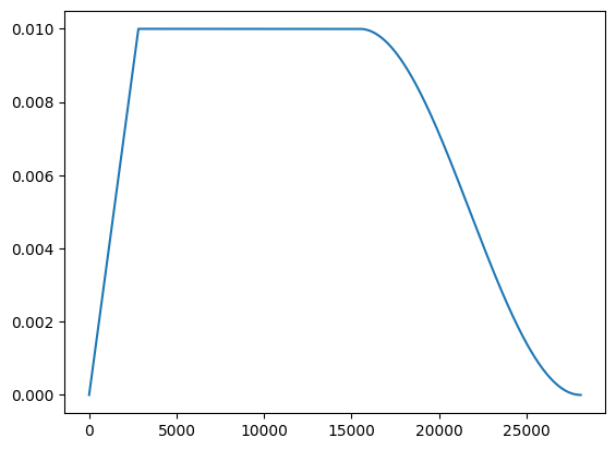
The schedule looks a as we expect.
Next let’s construct this optimizer:
total_images = 9000
total_steps = (total_images // BATCH_SIZE) * EPOCHS
warmup_steps = int(0.1 * total_steps)
hold_steps = int(0.45 * total_steps)
schedule = WarmUpCosineDecay(
    start_lr=0.05,
    target_lr=1e-2,
    warmup_steps=warmup_steps,
    total_steps=total_steps,
    hold=hold_steps,
)
optimizer = optimizers.SGD(
    weight_decay=5e-4,
    learning_rate=schedule,
    momentum=0.9,
)
At long last, we can now build our model and call fit()! Here, we directly instantiate our ResNetBackbone, specifying all architectural parameters, which gives us full control to tweak the architecture.
backbone = keras_hub.models.ResNetBackbone(
    input_conv_filters=[64],
    input_conv_kernel_sizes=[7],
    stackwise_num_filters=[64, 64, 64],
    stackwise_num_blocks=[2, 2, 2],
    stackwise_num_strides=[1, 2, 2],
    block_type="basic_block",
)
model = keras.Sequential(
    [
        backbone,
        keras.layers.GlobalMaxPooling2D(),
        keras.layers.Dropout(rate=0.5),
        keras.layers.Dense(101, activation="softmax"),
    ]
)
We employ label smoothing to prevent the model from overfitting to artifacts of our augmentation process.
loss = losses.CategoricalCrossentropy(label_smoothing=0.1)Let’s compile our model:
model.compile(
    loss=loss,
    optimizer=optimizer,
    metrics=[
        metrics.CategoricalAccuracy(),
        metrics.TopKCategoricalAccuracy(k=5),
    ],
)
and finally call fit().
model.fit(
    train_ds,
    epochs=EPOCHS,
    validation_data=eval_ds,
)
결과
1/96 [37m━━━━━━━━━━━━━━━━━━━━ 11:13 7s/step - categorical_accuracy: 0.0000e+00 - loss: 12.2444 - top_k_categorical_accuracy: 0.0938
96/96 ━━━━━━━━━━━━━━━━━━━━ 38s 327ms/step - categorical_accuracy: 0.0089 - loss: 8.5603 - top_k_categorical_accuracy: 0.0593 - val_categorical_accuracy: 0.0092 - val_loss: 5.7528 - val_top_k_categorical_accuracy: 0.0761
<keras.src.callbacks.history.History at 0x7f5b2892d190>Congratulations! You now know how to train a powerful image classifier from scratch using KerasHub. Depending on the availability of labeled data for your application, training from scratch may or may not be more powerful than using transfer learning in addition to the data augmentations discussed above. For smaller datasets, pretrained models generally produce high accuracy and faster convergence.
Conclusions
While image classification is perhaps the simplest problem in computer vision, the modern landscape has numerous complex components. Luckily, KerasHub offers robust, production-grade APIs to make assembling most of these components possible in one line of code. Through the use of KerasHub’s ImageClassifier API, pretrained weights, and Keras’ data augmentations you can assemble everything you need to train a powerful classifier in a few hundred lines of code!
As a follow up exercise, try fine tuning a KerasHub classifier on your own dataset!