비전 트랜스포머를 사용한 객체 감지
- 원본 링크 : https://keras.io/examples/vision/object_detection_using_vision_transformer/
- 최종 확인 : 2024-11-20
저자 : Karan V. Dave
생성일 : 2022/03/27
최종 편집일 : 2023/11/20
설명 : A simple Keras implementation of object detection using Vision Transformers.
Introduction
The article Vision Transformer (ViT) architecture by Alexey Dosovitskiy et al. demonstrates that a pure transformer applied directly to sequences of image patches can perform well on object detection tasks.
In this Keras example, we implement an object detection ViT and we train it on the Caltech 101 dataset to detect an airplane in the given image.
Imports and setup
import os

os.environ["KERAS_BACKEND"] = "jax"  # @param ["tensorflow", "jax", "torch"]


import numpy as np
import keras
from keras import layers
from keras import ops
import matplotlib.pyplot as plt
import numpy as np
import cv2
import os
import scipy.io
import shutil
Prepare dataset
We use the Caltech 101 Dataset.
# Path to images and annotations
path_images = "./101_ObjectCategories/airplanes/"
path_annot = "./Annotations/Airplanes_Side_2/"

path_to_downloaded_file = keras.utils.get_file(
    fname="caltech_101_zipped",
    origin="https://data.caltech.edu/records/mzrjq-6wc02/files/caltech-101.zip",
    extract=True,
    archive_format="zip",  # downloaded file format
    cache_dir="/",  # cache and extract in current directory
)
download_base_dir = os.path.dirname(path_to_downloaded_file)

# Extracting tar files found inside main zip file
shutil.unpack_archive(
    os.path.join(download_base_dir, "caltech-101", "101_ObjectCategories.tar.gz"), "."
)
shutil.unpack_archive(
    os.path.join(download_base_dir, "caltech-101", "Annotations.tar"), "."
)

# list of paths to images and annotations
image_paths = [
    f for f in os.listdir(path_images) if os.path.isfile(os.path.join(path_images, f))
]
annot_paths = [
    f for f in os.listdir(path_annot) if os.path.isfile(os.path.join(path_annot, f))
]

image_paths.sort()
annot_paths.sort()

image_size = 224  # resize input images to this size

images, targets = [], []

# loop over the annotations and images, preprocess them and store in lists
for i in range(0, len(annot_paths)):
    # Access bounding box coordinates
    annot = scipy.io.loadmat(path_annot + annot_paths[i])["box_coord"][0]

    top_left_x, top_left_y = annot[2], annot[0]
    bottom_right_x, bottom_right_y = annot[3], annot[1]

    image = keras.utils.load_img(
        path_images + image_paths[i],
    )
    (w, h) = image.size[:2]

    # resize images
    image = image.resize((image_size, image_size))

    # convert image to array and append to list
    images.append(keras.utils.img_to_array(image))

    # apply relative scaling to bounding boxes as per given image and append to list
    targets.append(
        (
            float(top_left_x) / w,
            float(top_left_y) / h,
            float(bottom_right_x) / w,
            float(bottom_right_y) / h,
        )
    )

# Convert the list to numpy array, split to train and test dataset
(x_train), (y_train) = (
    np.asarray(images[: int(len(images) * 0.8)]),
    np.asarray(targets[: int(len(targets) * 0.8)]),
)
(x_test), (y_test) = (
    np.asarray(images[int(len(images) * 0.8) :]),
    np.asarray(targets[int(len(targets) * 0.8) :]),
)
Implement multilayer-perceptron (MLP)
We use the code from the Keras example Image classification with Vision Transformer as a reference.
def mlp(x, hidden_units, dropout_rate):
    for units in hidden_units:
        x = layers.Dense(units, activation=keras.activations.gelu)(x)
        x = layers.Dropout(dropout_rate)(x)
    return x
Implement the patch creation layer
class Patches(layers.Layer):
    def __init__(self, patch_size):
        super().__init__()
        self.patch_size = patch_size

    def call(self, images):
        input_shape = ops.shape(images)
        batch_size = input_shape[0]
        height = input_shape[1]
        width = input_shape[2]
        channels = input_shape[3]
        num_patches_h = height // self.patch_size
        num_patches_w = width // self.patch_size
        patches = keras.ops.image.extract_patches(images, size=self.patch_size)
        patches = ops.reshape(
            patches,
            (
                batch_size,
                num_patches_h * num_patches_w,
                self.patch_size * self.patch_size * channels,
            ),
        )
        return patches

    def get_config(self):
        config = super().get_config()
        config.update({"patch_size": self.patch_size})
        return config
Display patches for an input image
patch_size = 32  # Size of the patches to be extracted from the input images

plt.figure(figsize=(4, 4))
plt.imshow(x_train[0].astype("uint8"))
plt.axis("off")

patches = Patches(patch_size)(np.expand_dims(x_train[0], axis=0))
print(f"Image size: {image_size} X {image_size}")
print(f"Patch size: {patch_size} X {patch_size}")
print(f"{patches.shape[1]} patches per image \n{patches.shape[-1]} elements per patch")


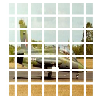
n = int(np.sqrt(patches.shape[1]))
plt.figure(figsize=(4, 4))
for i, patch in enumerate(patches[0]):
    ax = plt.subplot(n, n, i + 1)
    patch_img = ops.reshape(patch, (patch_size, patch_size, 3))
    plt.imshow(ops.convert_to_numpy(patch_img).astype("uint8"))
    plt.axis("off")
결과
Image size: 224 X 224
Patch size: 32 X 32
49 patches per image
3072 elements per patch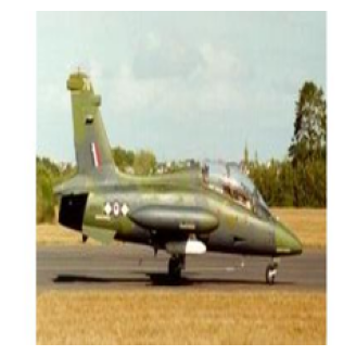
Implement the patch encoding layer
The PatchEncoder layer linearly transforms a patch by projecting it into a vector of size projection_dim. It also adds a learnable position embedding to the projected vector.
class PatchEncoder(layers.Layer):
    def __init__(self, num_patches, projection_dim):
        super().__init__()
        self.num_patches = num_patches
        self.projection = layers.Dense(units=projection_dim)
        self.position_embedding = layers.Embedding(
            input_dim=num_patches, output_dim=projection_dim
        )

    # Override function to avoid error while saving model
    def get_config(self):
        config = super().get_config().copy()
        config.update(
            {
                "input_shape": input_shape,
                "patch_size": patch_size,
                "num_patches": num_patches,
                "projection_dim": projection_dim,
                "num_heads": num_heads,
                "transformer_units": transformer_units,
                "transformer_layers": transformer_layers,
                "mlp_head_units": mlp_head_units,
            }
        )
        return config

    def call(self, patch):
        positions = ops.expand_dims(
            ops.arange(start=0, stop=self.num_patches, step=1), axis=0
        )
        projected_patches = self.projection(patch)
        encoded = projected_patches + self.position_embedding(positions)
        return encoded
Build the ViT model
The ViT model has multiple Transformer blocks. The MultiHeadAttention layer is used for self-attention, applied to the sequence of image patches. The encoded patches (skip connection) and self-attention layer outputs are normalized and fed into a multilayer perceptron (MLP). The model outputs four dimensions representing the bounding box coordinates of an object.
def create_vit_object_detector(
    input_shape,
    patch_size,
    num_patches,
    projection_dim,
    num_heads,
    transformer_units,
    transformer_layers,
    mlp_head_units,
):
    inputs = keras.Input(shape=input_shape)
    # Create patches
    patches = Patches(patch_size)(inputs)
    # Encode patches
    encoded_patches = PatchEncoder(num_patches, projection_dim)(patches)

    # Create multiple layers of the Transformer block.
    for _ in range(transformer_layers):
        # Layer normalization 1.
        x1 = layers.LayerNormalization(epsilon=1e-6)(encoded_patches)
        # Create a multi-head attention layer.
        attention_output = layers.MultiHeadAttention(
            num_heads=num_heads, key_dim=projection_dim, dropout=0.1
        )(x1, x1)
        # Skip connection 1.
        x2 = layers.Add()([attention_output, encoded_patches])
        # Layer normalization 2.
        x3 = layers.LayerNormalization(epsilon=1e-6)(x2)
        # MLP
        x3 = mlp(x3, hidden_units=transformer_units, dropout_rate=0.1)
        # Skip connection 2.
        encoded_patches = layers.Add()([x3, x2])

    # Create a [batch_size, projection_dim] tensor.
    representation = layers.LayerNormalization(epsilon=1e-6)(encoded_patches)
    representation = layers.Flatten()(representation)
    representation = layers.Dropout(0.3)(representation)
    # Add MLP.
    features = mlp(representation, hidden_units=mlp_head_units, dropout_rate=0.3)

    bounding_box = layers.Dense(4)(
        features
    )  # Final four neurons that output bounding box

    # return Keras model.
    return keras.Model(inputs=inputs, outputs=bounding_box)
Run the experiment
def run_experiment(model, learning_rate, weight_decay, batch_size, num_epochs):
    optimizer = keras.optimizers.AdamW(
        learning_rate=learning_rate, weight_decay=weight_decay
    )

    # Compile model.
    model.compile(optimizer=optimizer, loss=keras.losses.MeanSquaredError())

    checkpoint_filepath = "vit_object_detector.weights.h5"
    checkpoint_callback = keras.callbacks.ModelCheckpoint(
        checkpoint_filepath,
        monitor="val_loss",
        save_best_only=True,
        save_weights_only=True,
    )

    history = model.fit(
        x=x_train,
        y=y_train,
        batch_size=batch_size,
        epochs=num_epochs,
        validation_split=0.1,
        callbacks=[
            checkpoint_callback,
            keras.callbacks.EarlyStopping(monitor="val_loss", patience=10),
        ],
    )

    return history


input_shape = (image_size, image_size, 3)  # input image shape
learning_rate = 0.001
weight_decay = 0.0001
batch_size = 32
num_epochs = 100
num_patches = (image_size // patch_size) ** 2
projection_dim = 64
num_heads = 4
# Size of the transformer layers
transformer_units = [
    projection_dim * 2,
    projection_dim,
]
transformer_layers = 4
mlp_head_units = [2048, 1024, 512, 64, 32]  # Size of the dense layers


history = []
num_patches = (image_size // patch_size) ** 2

vit_object_detector = create_vit_object_detector(
    input_shape,
    patch_size,
    num_patches,
    projection_dim,
    num_heads,
    transformer_units,
    transformer_layers,
    mlp_head_units,
)

# Train model
history = run_experiment(
    vit_object_detector, learning_rate, weight_decay, batch_size, num_epochs
)


def plot_history(item):
    plt.plot(history.history[item], label=item)
    plt.plot(history.history["val_" + item], label="val_" + item)
    plt.xlabel("Epochs")
    plt.ylabel(item)
    plt.title("Train and Validation {} Over Epochs".format(item), fontsize=14)
    plt.legend()
    plt.grid()
    plt.show()


plot_history("loss")
결과
Epoch 1/100
 18/18 ━━━━━━━━━━━━━━━━━━━━ 9s 109ms/step - loss: 1.2097 - val_loss: 0.3468
Epoch 2/100
 18/18 ━━━━━━━━━━━━━━━━━━━━ 0s 25ms/step - loss: 0.4260 - val_loss: 0.3102
Epoch 3/100
 18/18 ━━━━━━━━━━━━━━━━━━━━ 0s 25ms/step - loss: 0.3268 - val_loss: 0.2727
Epoch 4/100
 18/18 ━━━━━━━━━━━━━━━━━━━━ 0s 25ms/step - loss: 0.2815 - val_loss: 0.2391
Epoch 5/100
 18/18 ━━━━━━━━━━━━━━━━━━━━ 0s 25ms/step - loss: 0.2290 - val_loss: 0.1735
Epoch 6/100
 18/18 ━━━━━━━━━━━━━━━━━━━━ 0s 24ms/step - loss: 0.1870 - val_loss: 0.1055
Epoch 7/100
 18/18 ━━━━━━━━━━━━━━━━━━━━ 0s 25ms/step - loss: 0.1401 - val_loss: 0.0610
Epoch 8/100
 18/18 ━━━━━━━━━━━━━━━━━━━━ 0s 25ms/step - loss: 0.1122 - val_loss: 0.0274
Epoch 9/100
 18/18 ━━━━━━━━━━━━━━━━━━━━ 0s 8ms/step - loss: 0.0924 - val_loss: 0.0296
Epoch 10/100
 18/18 ━━━━━━━━━━━━━━━━━━━━ 0s 24ms/step - loss: 0.0765 - val_loss: 0.0139
Epoch 11/100
 18/18 ━━━━━━━━━━━━━━━━━━━━ 0s 25ms/step - loss: 0.0597 - val_loss: 0.0111
Epoch 12/100
 18/18 ━━━━━━━━━━━━━━━━━━━━ 0s 25ms/step - loss: 0.0540 - val_loss: 0.0101
Epoch 13/100
 18/18 ━━━━━━━━━━━━━━━━━━━━ 0s 24ms/step - loss: 0.0432 - val_loss: 0.0053
Epoch 14/100
 18/18 ━━━━━━━━━━━━━━━━━━━━ 0s 24ms/step - loss: 0.0380 - val_loss: 0.0052
Epoch 15/100
 18/18 ━━━━━━━━━━━━━━━━━━━━ 0s 25ms/step - loss: 0.0334 - val_loss: 0.0030
Epoch 16/100
 18/18 ━━━━━━━━━━━━━━━━━━━━ 0s 25ms/step - loss: 0.0283 - val_loss: 0.0021
Epoch 17/100
 18/18 ━━━━━━━━━━━━━━━━━━━━ 0s 24ms/step - loss: 0.0228 - val_loss: 0.0012
Epoch 18/100
 18/18 ━━━━━━━━━━━━━━━━━━━━ 0s 8ms/step - loss: 0.0244 - val_loss: 0.0017
Epoch 19/100
 18/18 ━━━━━━━━━━━━━━━━━━━━ 0s 8ms/step - loss: 0.0195 - val_loss: 0.0016
Epoch 20/100
 18/18 ━━━━━━━━━━━━━━━━━━━━ 0s 8ms/step - loss: 0.0189 - val_loss: 0.0020
Epoch 21/100
 18/18 ━━━━━━━━━━━━━━━━━━━━ 0s 8ms/step - loss: 0.0191 - val_loss: 0.0019
Epoch 22/100
 18/18 ━━━━━━━━━━━━━━━━━━━━ 0s 8ms/step - loss: 0.0174 - val_loss: 0.0016
Epoch 23/100
 18/18 ━━━━━━━━━━━━━━━━━━━━ 0s 8ms/step - loss: 0.0157 - val_loss: 0.0020
Epoch 24/100
 18/18 ━━━━━━━━━━━━━━━━━━━━ 0s 8ms/step - loss: 0.0157 - val_loss: 0.0015
Epoch 25/100
 18/18 ━━━━━━━━━━━━━━━━━━━━ 0s 8ms/step - loss: 0.0139 - val_loss: 0.0023
Epoch 26/100
 18/18 ━━━━━━━━━━━━━━━━━━━━ 0s 8ms/step - loss: 0.0130 - val_loss: 0.0017
Epoch 27/100
 18/18 ━━━━━━━━━━━━━━━━━━━━ 0s 8ms/step - loss: 0.0157 - val_loss: 0.0014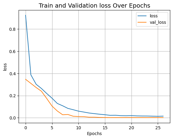
Evaluate the model
import matplotlib.patches as patches

# Saves the model in current path
vit_object_detector.save("vit_object_detector.keras")


# To calculate IoU (intersection over union, given two bounding boxes)
def bounding_box_intersection_over_union(box_predicted, box_truth):
    # get (x, y) coordinates of intersection of bounding boxes
    top_x_intersect = max(box_predicted[0], box_truth[0])
    top_y_intersect = max(box_predicted[1], box_truth[1])
    bottom_x_intersect = min(box_predicted[2], box_truth[2])
    bottom_y_intersect = min(box_predicted[3], box_truth[3])

    # calculate area of the intersection bb (bounding box)
    intersection_area = max(0, bottom_x_intersect - top_x_intersect + 1) * max(
        0, bottom_y_intersect - top_y_intersect + 1
    )

    # calculate area of the prediction bb and ground-truth bb
    box_predicted_area = (box_predicted[2] - box_predicted[0] + 1) * (
        box_predicted[3] - box_predicted[1] + 1
    )
    box_truth_area = (box_truth[2] - box_truth[0] + 1) * (
        box_truth[3] - box_truth[1] + 1
    )

    # calculate intersection over union by taking intersection
    # area and dividing it by the sum of predicted bb and ground truth
    # bb areas subtracted by  the interesection area

    # return ioU
    return intersection_area / float(
        box_predicted_area + box_truth_area - intersection_area
    )


i, mean_iou = 0, 0

# Compare results for 10 images in the test set
for input_image in x_test[:10]:
    fig, (ax1, ax2) = plt.subplots(1, 2, figsize=(15, 15))
    im = input_image

    # Display the image
    ax1.imshow(im.astype("uint8"))
    ax2.imshow(im.astype("uint8"))

    input_image = cv2.resize(
        input_image, (image_size, image_size), interpolation=cv2.INTER_AREA
    )
    input_image = np.expand_dims(input_image, axis=0)
    preds = vit_object_detector.predict(input_image)[0]

    (h, w) = (im).shape[0:2]

    top_left_x, top_left_y = int(preds[0] * w), int(preds[1] * h)

    bottom_right_x, bottom_right_y = int(preds[2] * w), int(preds[3] * h)

    box_predicted = [top_left_x, top_left_y, bottom_right_x, bottom_right_y]
    # Create the bounding box
    rect = patches.Rectangle(
        (top_left_x, top_left_y),
        bottom_right_x - top_left_x,
        bottom_right_y - top_left_y,
        facecolor="none",
        edgecolor="red",
        linewidth=1,
    )
    # Add the bounding box to the image
    ax1.add_patch(rect)
    ax1.set_xlabel(
        "Predicted: "
        + str(top_left_x)
        + ", "
        + str(top_left_y)
        + ", "
        + str(bottom_right_x)
        + ", "
        + str(bottom_right_y)
    )

    top_left_x, top_left_y = int(y_test[i][0] * w), int(y_test[i][1] * h)

    bottom_right_x, bottom_right_y = int(y_test[i][2] * w), int(y_test[i][3] * h)

    box_truth = top_left_x, top_left_y, bottom_right_x, bottom_right_y

    mean_iou += bounding_box_intersection_over_union(box_predicted, box_truth)
    # Create the bounding box
    rect = patches.Rectangle(
        (top_left_x, top_left_y),
        bottom_right_x - top_left_x,
        bottom_right_y - top_left_y,
        facecolor="none",
        edgecolor="red",
        linewidth=1,
    )
    # Add the bounding box to the image
    ax2.add_patch(rect)
    ax2.set_xlabel(
        "Target: "
        + str(top_left_x)
        + ", "
        + str(top_left_y)
        + ", "
        + str(bottom_right_x)
        + ", "
        + str(bottom_right_y)
        + "\n"
        + "IoU"
        + str(bounding_box_intersection_over_union(box_predicted, box_truth))
    )
    i = i + 1

print("mean_iou: " + str(mean_iou / len(x_test[:10])))
plt.show()
결과
 1/1 ━━━━━━━━━━━━━━━━━━━━ 1s 1s/step
 1/1 ━━━━━━━━━━━━━━━━━━━━ 0s 1ms/step
 1/1 ━━━━━━━━━━━━━━━━━━━━ 0s 1ms/step
 1/1 ━━━━━━━━━━━━━━━━━━━━ 0s 2ms/step
 1/1 ━━━━━━━━━━━━━━━━━━━━ 0s 1ms/step
 1/1 ━━━━━━━━━━━━━━━━━━━━ 0s 1ms/step
 1/1 ━━━━━━━━━━━━━━━━━━━━ 0s 1ms/step
 1/1 ━━━━━━━━━━━━━━━━━━━━ 0s 1ms/step
 1/1 ━━━━━━━━━━━━━━━━━━━━ 0s 2ms/step
 1/1 ━━━━━━━━━━━━━━━━━━━━ 0s 1ms/step
mean_iou: 0.9092338486331416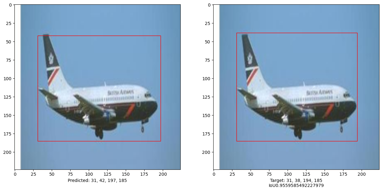

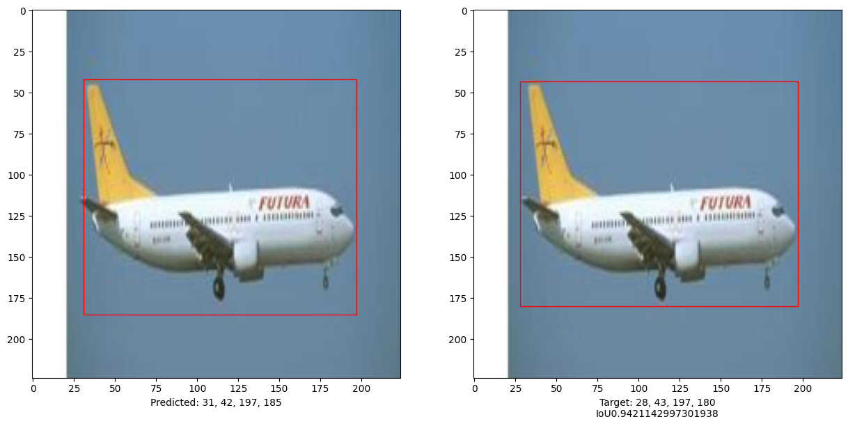
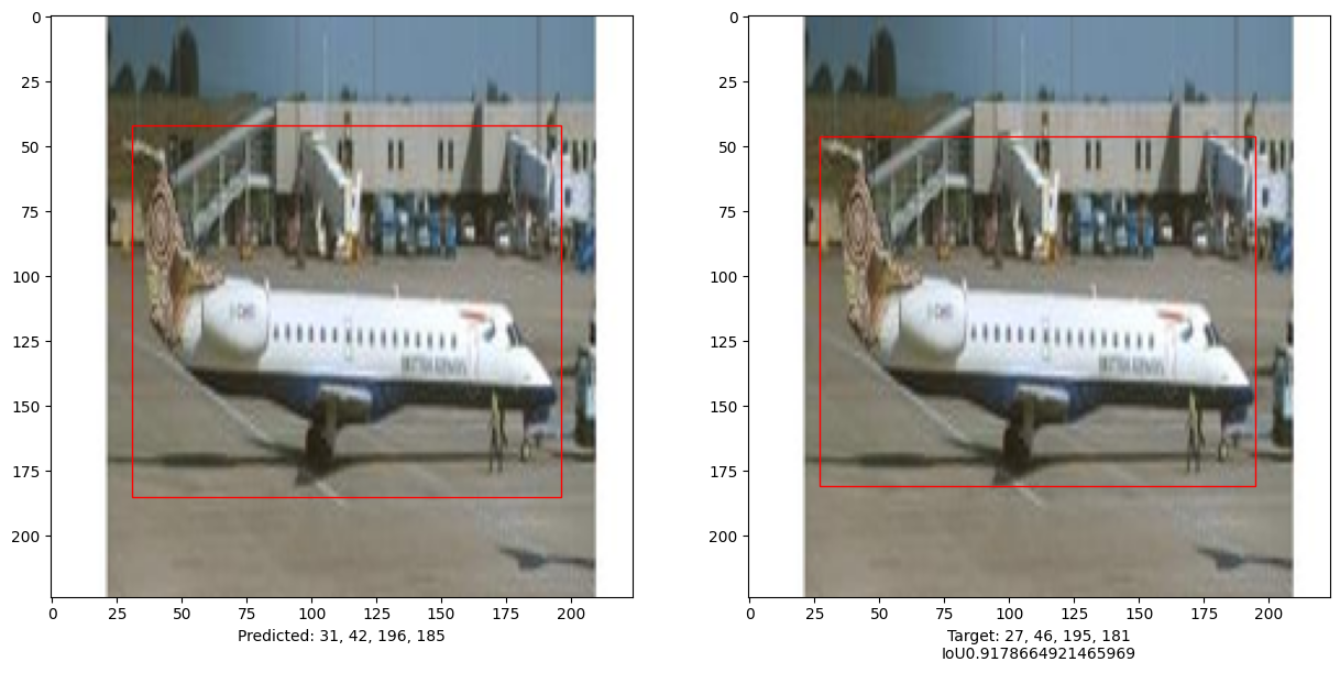
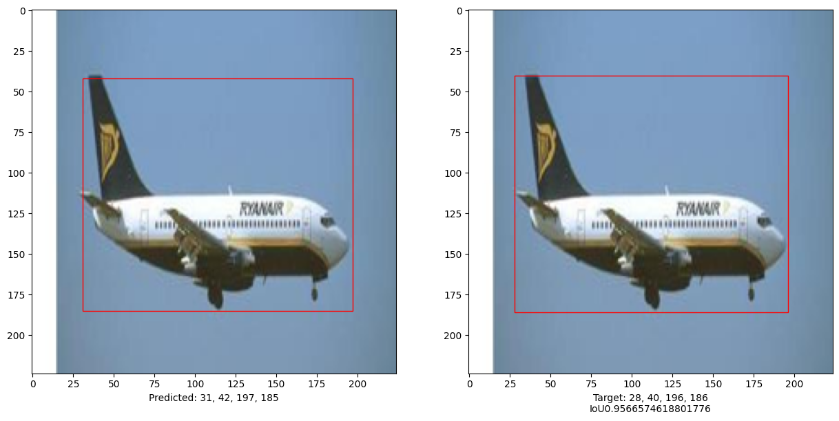
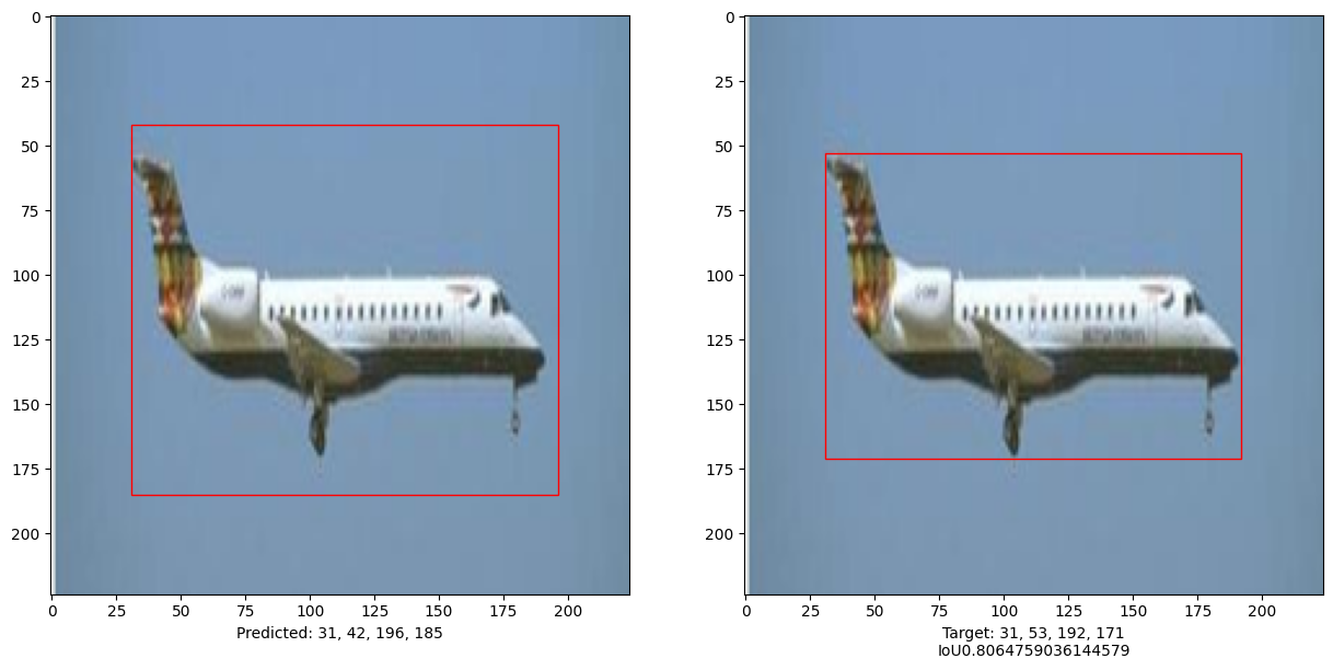
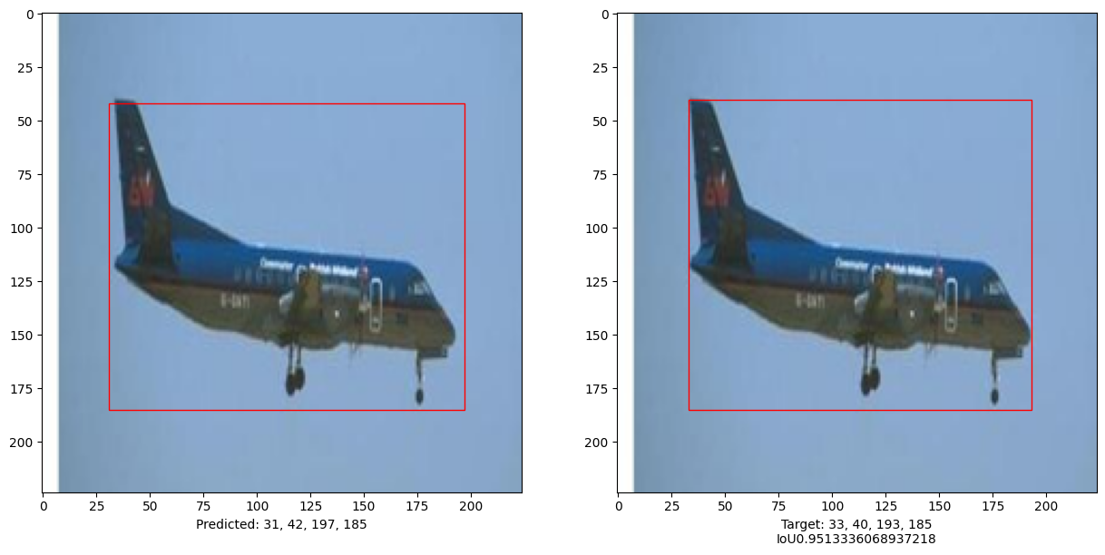
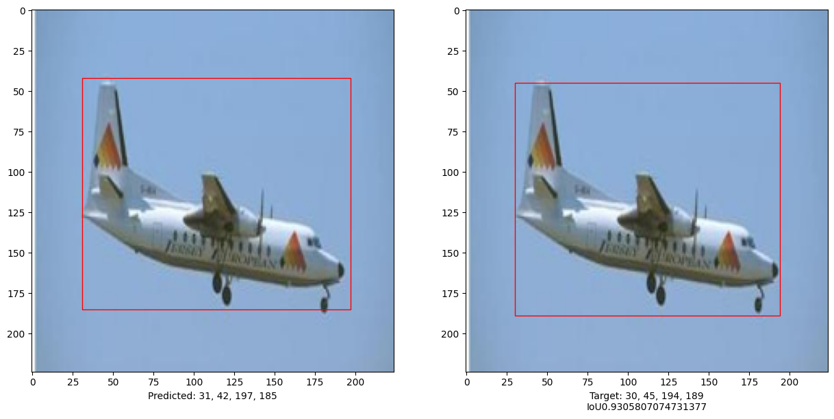
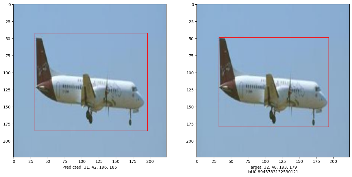
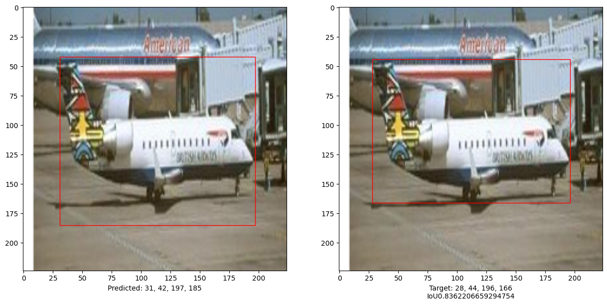
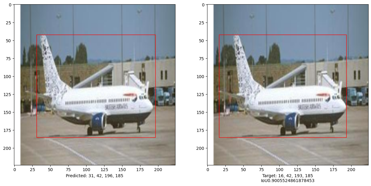
This example demonstrates that a pure Transformer can be trained to predict the bounding boxes of an object in a given image, thus extending the use of Transformers to object detection tasks. The model can be improved further by tuning hyper-parameters and pre-training.