AdaMatch를 통한 반지도(Semi-supervision) 및 도메인 적응
- 원본 링크 : https://keras.io/examples/vision/adamatch/
- 최종 확인 : 2024-11-21
저자 : Sayak Paul
생성일 : 2021/06/19
최종 편집일 : 2021/06/19
설명 : Unifying semi-supervised learning and unsupervised domain adaptation with AdaMatch.
Introduction
In this example, we will implement the AdaMatch algorithm, proposed in AdaMatch: A Unified Approach to Semi-Supervised Learning and Domain Adaptation by Berthelot et al. It sets a new state-of-the-art in unsupervised domain adaptation (as of June 2021). AdaMatch is particularly interesting because it unifies semi-supervised learning (SSL) and unsupervised domain adaptation (UDA) under one framework. It thereby provides a way to perform semi-supervised domain adaptation (SSDA).
This example requires TensorFlow 2.5 or higher, as well as TensorFlow Models, which can be installed using the following command:
!pip install -q tf-models-official==2.9.2Before we proceed, let’s review a few preliminary concepts underlying this example.
Preliminaries
In semi-supervised learning (SSL), we use a small amount of labeled data to train models on a bigger unlabeled dataset. Popular semi-supervised learning methods for computer vision include FixMatch, MixMatch, Noisy Student Training, etc. You can refer to this example to get an idea of what a standard SSL workflow looks like.
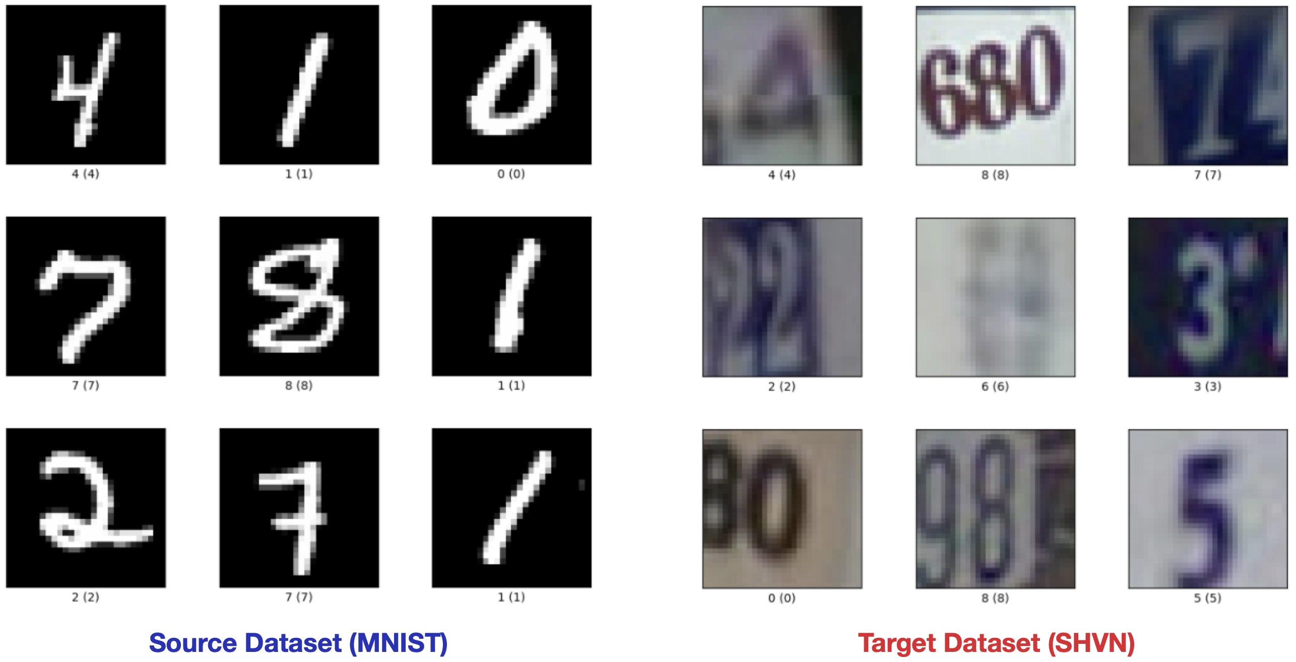
In unsupervised domain adaptation, we have access to a source labeled dataset and a target unlabeled dataset. Then the task is to learn a model that can generalize well to the target dataset. The source and the target datasets vary in terms of distribution. The following figure provides an illustration of this idea. In the present example, we use the MNIST dataset as the source dataset, while the target dataset is SVHN, which consists of images of house numbers. Both datasets have various varying factors in terms of texture, viewpoint, appearance, etc.: their domains, or distributions, are different from one another.

Popular domain adaptation algorithms in deep learning include Deep CORAL, Moment Matching, etc.
Setup
import tensorflow as tf

tf.random.set_seed(42)

import numpy as np

from tensorflow import keras
from tensorflow.keras import layers
from tensorflow.keras import regularizers
from keras_cv.layers import RandAugment

import tensorflow_datasets as tfds

tfds.disable_progress_bar()
Prepare the data
# MNIST
(
    (mnist_x_train, mnist_y_train),
    (mnist_x_test, mnist_y_test),
) = keras.datasets.mnist.load_data()

# Add a channel dimension
mnist_x_train = tf.expand_dims(mnist_x_train, -1)
mnist_x_test = tf.expand_dims(mnist_x_test, -1)

# Convert the labels to one-hot encoded vectors
mnist_y_train = tf.one_hot(mnist_y_train, 10).numpy()

# SVHN
svhn_train, svhn_test = tfds.load(
    "svhn_cropped", split=["train", "test"], as_supervised=True
)
Define constants and hyperparameters
RESIZE_TO = 32

SOURCE_BATCH_SIZE = 64
TARGET_BATCH_SIZE = 3 * SOURCE_BATCH_SIZE  # Reference: Section 3.2
EPOCHS = 10
STEPS_PER_EPOCH = len(mnist_x_train) // SOURCE_BATCH_SIZE
TOTAL_STEPS = EPOCHS * STEPS_PER_EPOCH

AUTO = tf.data.AUTOTUNE
LEARNING_RATE = 0.03

WEIGHT_DECAY = 0.0005
INIT = "he_normal"
DEPTH = 28
WIDTH_MULT = 2
Data augmentation utilities
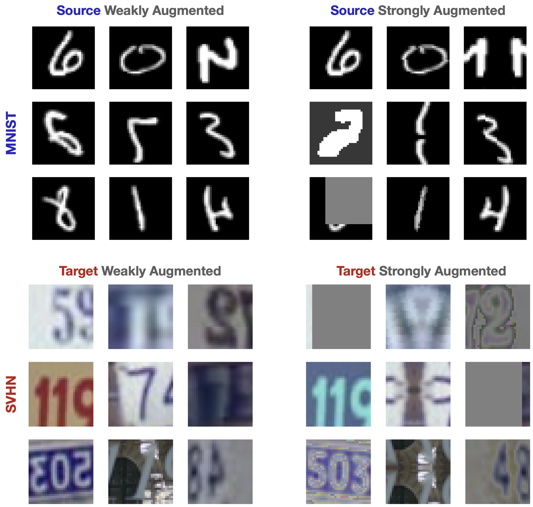
A standard element of SSL algorithms is to feed weakly and strongly augmented versions of the same images to the learning model to make its predictions consistent. For strong augmentation, RandAugment is a standard choice. For weak augmentation, we will use horizontal flipping and random cropping.
# Initialize `RandAugment` object with 2 layers of
# augmentation transforms and strength of 5.
augmenter = RandAugment(value_range=(0, 255), augmentations_per_image=2, magnitude=0.5)


def weak_augment(image, source=True):
    if image.dtype != tf.float32:
        image = tf.cast(image, tf.float32)

    # MNIST images are grayscale, this is why we first convert them to
    # RGB images.
    if source:
        image = tf.image.resize_with_pad(image, RESIZE_TO, RESIZE_TO)
        image = tf.tile(image, [1, 1, 3])
    image = tf.image.random_flip_left_right(image)
    image = tf.image.random_crop(image, (RESIZE_TO, RESIZE_TO, 3))
    return image


def strong_augment(image, source=True):
    if image.dtype != tf.float32:
        image = tf.cast(image, tf.float32)

    if source:
        image = tf.image.resize_with_pad(image, RESIZE_TO, RESIZE_TO)
        image = tf.tile(image, [1, 1, 3])
    image = augmenter(image)
    return image
Data loading utilities
def create_individual_ds(ds, aug_func, source=True):
    if source:
        batch_size = SOURCE_BATCH_SIZE
    else:
        # During training 3x more target unlabeled samples are shown
        # to the model in AdaMatch (Section 3.2 of the paper).
        batch_size = TARGET_BATCH_SIZE
    ds = ds.shuffle(batch_size * 10, seed=42)

    if source:
        ds = ds.map(lambda x, y: (aug_func(x), y), num_parallel_calls=AUTO)
    else:
        ds = ds.map(lambda x, y: (aug_func(x, False), y), num_parallel_calls=AUTO)

    ds = ds.batch(batch_size).prefetch(AUTO)
    return ds
_w and _s suffixes denote weak and strong respectively.
source_ds = tf.data.Dataset.from_tensor_slices((mnist_x_train, mnist_y_train))
source_ds_w = create_individual_ds(source_ds, weak_augment)
source_ds_s = create_individual_ds(source_ds, strong_augment)
final_source_ds = tf.data.Dataset.zip((source_ds_w, source_ds_s))

target_ds_w = create_individual_ds(svhn_train, weak_augment, source=False)
target_ds_s = create_individual_ds(svhn_train, strong_augment, source=False)
final_target_ds = tf.data.Dataset.zip((target_ds_w, target_ds_s))
Here’s what a single image batch looks like:

Loss computation utilities
def compute_loss_source(source_labels, logits_source_w, logits_source_s):
    loss_func = keras.losses.CategoricalCrossentropy(from_logits=True)
    # First compute the losses between original source labels and
    # predictions made on the weakly and strongly augmented versions
    # of the same images.
    w_loss = loss_func(source_labels, logits_source_w)
    s_loss = loss_func(source_labels, logits_source_s)
    return w_loss + s_loss


def compute_loss_target(target_pseudo_labels_w, logits_target_s, mask):
    loss_func = keras.losses.CategoricalCrossentropy(from_logits=True, reduction="none")
    target_pseudo_labels_w = tf.stop_gradient(target_pseudo_labels_w)
    # For calculating loss for the target samples, we treat the pseudo labels
    # as the ground-truth. These are not considered during backpropagation
    # which is a standard SSL practice.
    target_loss = loss_func(target_pseudo_labels_w, logits_target_s)

    # More on `mask` later.
    mask = tf.cast(mask, target_loss.dtype)
    target_loss *= mask
    return tf.reduce_mean(target_loss, 0)
Subclassed model for AdaMatch training
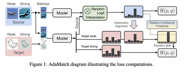
The figure below presents the overall workflow of AdaMatch (taken from the original paper):

Here’s a brief step-by-step breakdown of the workflow:
- We first retrieve the weakly and strongly augmented pairs of images from the source and target datasets.
- We prepare two concatenated copies: i. One where both pairs are concatenated. ii. One where only the source data image pair is concatenated.
- We run two forward passes through the model: i. The first forward pass uses the concatenated copy obtained from 2.i. In this forward pass, the Batch Normalization statistics are updated. ii. In the second forward pass, we only use the concatenated copy obtained from 2.ii. Batch Normalization layers are run in inference mode.
- The respective logits are computed for both the forward passes.
- The logits go through a series of transformations, introduced in the paper (which we will discuss shortly).
- We compute the loss and update the gradients of the underlying model.
class AdaMatch(keras.Model):
    def __init__(self, model, total_steps, tau=0.9):
        super().__init__()
        self.model = model
        self.tau = tau  # Denotes the confidence threshold
        self.loss_tracker = tf.keras.metrics.Mean(name="loss")
        self.total_steps = total_steps
        self.current_step = tf.Variable(0, dtype="int64")

    @property
    def metrics(self):
        return [self.loss_tracker]

    # This is a warmup schedule to update the weight of the
    # loss contributed by the target unlabeled samples. More
    # on this in the text.
    def compute_mu(self):
        pi = tf.constant(np.pi, dtype="float32")
        step = tf.cast(self.current_step, dtype="float32")
        return 0.5 - tf.cos(tf.math.minimum(pi, (2 * pi * step) / self.total_steps)) / 2

    def train_step(self, data):
        ## Unpack and organize the data ##
        source_ds, target_ds = data
        (source_w, source_labels), (source_s, _) = source_ds
        (
            (target_w, _),
            (target_s, _),
        ) = target_ds  # Notice that we are NOT using any labels here.

        combined_images = tf.concat([source_w, source_s, target_w, target_s], 0)
        combined_source = tf.concat([source_w, source_s], 0)

        total_source = tf.shape(combined_source)[0]
        total_target = tf.shape(tf.concat([target_w, target_s], 0))[0]

        with tf.GradientTape() as tape:
            ## Forward passes ##
            combined_logits = self.model(combined_images, training=True)
            z_d_prime_source = self.model(
                combined_source, training=False
            )  # No BatchNorm update.
            z_prime_source = combined_logits[:total_source]

            ## 1. Random logit interpolation for the source images ##
            lambd = tf.random.uniform((total_source, 10), 0, 1)
            final_source_logits = (lambd * z_prime_source) + (
                (1 - lambd) * z_d_prime_source
            )

            ## 2. Distribution alignment (only consider weakly augmented images) ##
            # Compute softmax for logits of the WEAKLY augmented SOURCE images.
            y_hat_source_w = tf.nn.softmax(final_source_logits[: tf.shape(source_w)[0]])

            # Extract logits for the WEAKLY augmented TARGET images and compute softmax.
            logits_target = combined_logits[total_source:]
            logits_target_w = logits_target[: tf.shape(target_w)[0]]
            y_hat_target_w = tf.nn.softmax(logits_target_w)

            # Align the target label distribution to that of the source.
            expectation_ratio = tf.reduce_mean(y_hat_source_w) / tf.reduce_mean(
                y_hat_target_w
            )
            y_tilde_target_w = tf.math.l2_normalize(
                y_hat_target_w * expectation_ratio, 1
            )

            ## 3. Relative confidence thresholding ##
            row_wise_max = tf.reduce_max(y_hat_source_w, axis=-1)
            final_sum = tf.reduce_mean(row_wise_max, 0)
            c_tau = self.tau * final_sum
            mask = tf.reduce_max(y_tilde_target_w, axis=-1) >= c_tau

            ## Compute losses (pay attention to the indexing) ##
            source_loss = compute_loss_source(
                source_labels,
                final_source_logits[: tf.shape(source_w)[0]],
                final_source_logits[tf.shape(source_w)[0] :],
            )
            target_loss = compute_loss_target(
                y_tilde_target_w, logits_target[tf.shape(target_w)[0] :], mask
            )

            t = self.compute_mu()  # Compute weight for the target loss
            total_loss = source_loss + (t * target_loss)
            self.current_step.assign_add(
                1
            )  # Update current training step for the scheduler

        gradients = tape.gradient(total_loss, self.model.trainable_variables)
        self.optimizer.apply_gradients(zip(gradients, self.model.trainable_variables))

        self.loss_tracker.update_state(total_loss)
        return {"loss": self.loss_tracker.result()}
The authors introduce three improvements in the paper:
- In AdaMatch, we perform two forward passes, and only one of them is respsonsible for updating the Batch Normalization statistics. This is done to account for distribution shifts in the target dataset. In the other forward pass, we only use the source sample, and the Batch Normalization layers are run in inference mode. Logits for the source samples (weakly and strongly augmented versions) from these two passes are slightly different from one another because of how Batch Normalization layers are run. Final logits for the source samples are computed by linearly interpolating between these two different pairs of logits. This induces a form of consistency regularization. This step is referred to as random logit interpolation.
- Distribution alignment is used to align the source and target label distributions. This further helps the underlying model learn domain-invariant representations. In case of unsupervised domain adaptation, we don’t have access to any labels of the target dataset. This is why pseudo labels are generated from the underlying model.
- The underlying model generates pseudo-labels for the target samples. It’s likely that the model would make faulty predictions. Those can propagate back as we make progress in the training, and hurt the overall performance. To compensate for that, we filter the high-confidence predictions based on a threshold (hence the use of
maskinsidecompute_loss_target()). In AdaMatch, this threshold is relatively adjusted which is why it is called relative confidence thresholding.
For more details on these methods and to know how each of them contribute please refer to the paper.
About compute_mu():
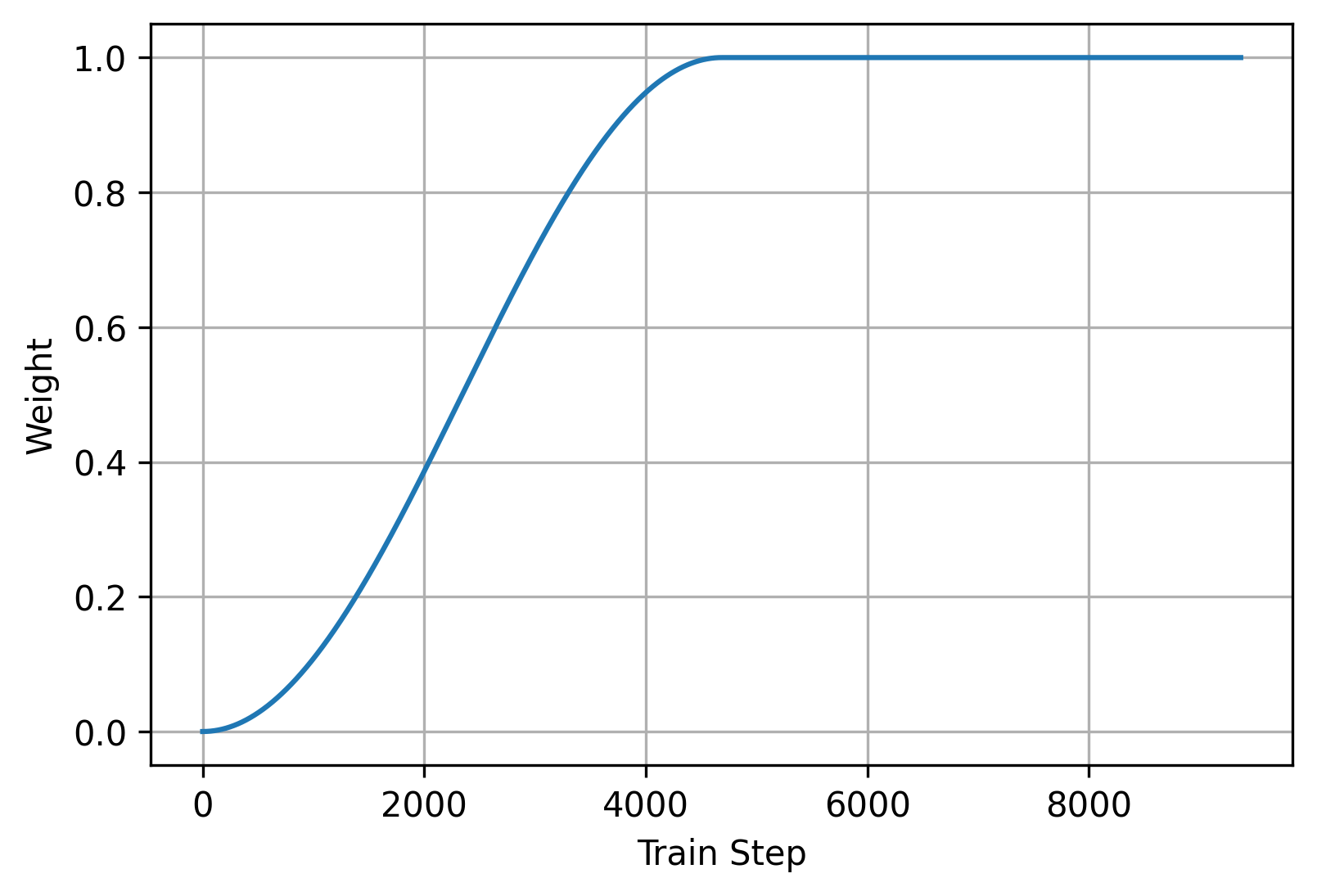
Rather than using a fixed scalar quantity, a varying scalar is used in AdaMatch. It denotes the weight of the loss contibuted by the target samples. Visually, the weight scheduler look like so:

This scheduler increases the weight of the target domain loss from 0 to 1 for the first half of the training. Then it keeps that weight at 1 for the second half of the training.
Instantiate a Wide-ResNet-28-2
The authors use a WideResNet-28-2 for the dataset pairs we are using in this example. Most of the following code has been referred from this script. Note that the following model has a scaling layer inside it that scales the pixel values to [0, 1].
def wide_basic(x, n_input_plane, n_output_plane, stride):
    conv_params = [[3, 3, stride, "same"], [3, 3, (1, 1), "same"]]

    n_bottleneck_plane = n_output_plane

    # Residual block
    for i, v in enumerate(conv_params):
        if i == 0:
            if n_input_plane != n_output_plane:
                x = layers.BatchNormalization()(x)
                x = layers.Activation("relu")(x)
                convs = x
            else:
                convs = layers.BatchNormalization()(x)
                convs = layers.Activation("relu")(convs)
            convs = layers.Conv2D(
                n_bottleneck_plane,
                (v[0], v[1]),
                strides=v[2],
                padding=v[3],
                kernel_initializer=INIT,
                kernel_regularizer=regularizers.l2(WEIGHT_DECAY),
                use_bias=False,
            )(convs)
        else:
            convs = layers.BatchNormalization()(convs)
            convs = layers.Activation("relu")(convs)
            convs = layers.Conv2D(
                n_bottleneck_plane,
                (v[0], v[1]),
                strides=v[2],
                padding=v[3],
                kernel_initializer=INIT,
                kernel_regularizer=regularizers.l2(WEIGHT_DECAY),
                use_bias=False,
            )(convs)

    # Shortcut connection: identity function or 1x1
    # convolutional
    #  (depends on difference between input & output shape - this
    #   corresponds to whether we are using the first block in
    #   each
    #   group; see `block_series()`).
    if n_input_plane != n_output_plane:
        shortcut = layers.Conv2D(
            n_output_plane,
            (1, 1),
            strides=stride,
            padding="same",
            kernel_initializer=INIT,
            kernel_regularizer=regularizers.l2(WEIGHT_DECAY),
            use_bias=False,
        )(x)
    else:
        shortcut = x

    return layers.Add()([convs, shortcut])


# Stacking residual units on the same stage
def block_series(x, n_input_plane, n_output_plane, count, stride):
    x = wide_basic(x, n_input_plane, n_output_plane, stride)
    for i in range(2, int(count + 1)):
        x = wide_basic(x, n_output_plane, n_output_plane, stride=1)
    return x


def get_network(image_size=32, num_classes=10):
    n = (DEPTH - 4) / 6
    n_stages = [16, 16 * WIDTH_MULT, 32 * WIDTH_MULT, 64 * WIDTH_MULT]

    inputs = keras.Input(shape=(image_size, image_size, 3))
    x = layers.Rescaling(scale=1.0 / 255)(inputs)

    conv1 = layers.Conv2D(
        n_stages[0],
        (3, 3),
        strides=1,
        padding="same",
        kernel_initializer=INIT,
        kernel_regularizer=regularizers.l2(WEIGHT_DECAY),
        use_bias=False,
    )(x)

    ## Add wide residual blocks ##

    conv2 = block_series(
        conv1,
        n_input_plane=n_stages[0],
        n_output_plane=n_stages[1],
        count=n,
        stride=(1, 1),
    )  # Stage 1

    conv3 = block_series(
        conv2,
        n_input_plane=n_stages[1],
        n_output_plane=n_stages[2],
        count=n,
        stride=(2, 2),
    )  # Stage 2

    conv4 = block_series(
        conv3,
        n_input_plane=n_stages[2],
        n_output_plane=n_stages[3],
        count=n,
        stride=(2, 2),
    )  # Stage 3

    batch_norm = layers.BatchNormalization()(conv4)
    relu = layers.Activation("relu")(batch_norm)

    # Classifier
    trunk_outputs = layers.GlobalAveragePooling2D()(relu)
    outputs = layers.Dense(
        num_classes, kernel_regularizer=regularizers.l2(WEIGHT_DECAY)
    )(trunk_outputs)

    return keras.Model(inputs, outputs)
We can now instantiate a Wide ResNet model like so. Note that the purpose of using a Wide ResNet here is to keep the implementation as close to the original one as possible.
wrn_model = get_network()
print(f"Model has {wrn_model.count_params()/1e6} Million parameters.")
결과
Model has 1.471226 Million parameters.Instantiate AdaMatch model and compile it
reduce_lr = keras.optimizers.schedules.CosineDecay(LEARNING_RATE, TOTAL_STEPS, 0.25)
optimizer = keras.optimizers.Adam(reduce_lr)

adamatch_trainer = AdaMatch(model=wrn_model, total_steps=TOTAL_STEPS)
adamatch_trainer.compile(optimizer=optimizer)
Model training
total_ds = tf.data.Dataset.zip((final_source_ds, final_target_ds))
adamatch_trainer.fit(total_ds, epochs=EPOCHS)
결과
Epoch 1/10
382/382 [==============================] - 155s 392ms/step - loss: 149259583488.0000
Epoch 2/10
382/382 [==============================] - 145s 379ms/step - loss: 2.0935
Epoch 3/10
382/382 [==============================] - 145s 380ms/step - loss: 1.7237
Epoch 4/10
382/382 [==============================] - 142s 370ms/step - loss: 1.9182
Epoch 5/10
382/382 [==============================] - 141s 367ms/step - loss: 2.9698
Epoch 6/10
382/382 [==============================] - 141s 368ms/step - loss: 3.2622
Epoch 7/10
382/382 [==============================] - 141s 367ms/step - loss: 2.9034
Epoch 8/10
382/382 [==============================] - 141s 368ms/step - loss: 3.2735
Epoch 9/10
382/382 [==============================] - 141s 369ms/step - loss: 3.9449
Epoch 10/10
382/382 [==============================] - 141s 369ms/step - loss: 3.5918

<keras.callbacks.History at 0x7f16eb261e20>
Evaluation on the target and source test sets
# Compile the AdaMatch model to yield accuracy.
adamatch_trained_model = adamatch_trainer.model
adamatch_trained_model.compile(metrics=keras.metrics.SparseCategoricalAccuracy())

# Score on the target test set.
svhn_test = svhn_test.batch(TARGET_BATCH_SIZE).prefetch(AUTO)
_, accuracy = adamatch_trained_model.evaluate(svhn_test)
print(f"Accuracy on target test set: {accuracy * 100:.2f}%")
결과
136/136 [==============================] - 4s 24ms/step - loss: 508.2073 - sparse_categorical_accuracy: 0.2408
Accuracy on target test set: 24.08%
With more training, this score improves. When this same network is trained with standard classification objective, it yields an accuracy of 7.20% which is significantly lower than what we got with AdaMatch. You can check out this notebook to learn more about the hyperparameters and other experimental details.
# Utility function for preprocessing the source test set.
def prepare_test_ds_source(image, label):
    image = tf.image.resize_with_pad(image, RESIZE_TO, RESIZE_TO)
    image = tf.tile(image, [1, 1, 3])
    return image, label


source_test_ds = tf.data.Dataset.from_tensor_slices((mnist_x_test, mnist_y_test))
source_test_ds = (
    source_test_ds.map(prepare_test_ds_source, num_parallel_calls=AUTO)
    .batch(TARGET_BATCH_SIZE)
    .prefetch(AUTO)
)

# Evaluation on the source test set.
_, accuracy = adamatch_trained_model.evaluate(source_test_ds)
print(f"Accuracy on source test set: {accuracy * 100:.2f}%")
결과
53/53 [==============================] - 2s 24ms/step - loss: 508.2072 - sparse_categorical_accuracy: 0.9736
Accuracy on source test set: 97.36%
You can reproduce the results by using these model weights.
Example available on HuggingFace
| Trained Model | Demo |
|---|---|
 |  |