Semantic Segmentation with KerasCV
- Original Link : https://keras.io/guides/keras_cv/semantic_segmentation_deeplab_v3_plus/
- Last Checked at : 2024-11-19
Author: Divyashree Sreepathihalli, Ian Stenbit
Date created: 2023/08/22
Last modified: 2023/08/24
Description: Train and use DeepLabv3+ segmentation model with KerasCV.

Background
Semantic segmentation is a type of computer vision task that involves assigning a class label such as person, bike, or background to each individual pixel of an image, effectively dividing the image into regions that correspond to different fobject classes or categories.
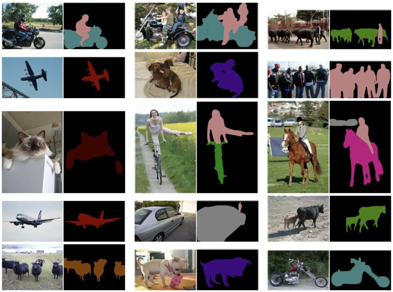
KerasCV offers the DeepLabv3+ model developed by Google for semantic segmentation. This guide demonstrates how to finetune and use DeepLabv3+ model for image semantic segmentaion with KerasCV. Its architecture that combines atrous convolutions, contextual information aggregation, and powerful backbones to achieve accurate and detailed semantic segmentation. The DeepLabv3+ model has been shown to achieve state-of-the-art results on a variety of image segmentation benchmarks.
References
Encoder-Decoder with Atrous Separable Convolution for Semantic Image Segmentation
Rethinking Atrous Convolution for Semantic Image Segmentation
Setup and Imports
Let’s install the dependencies and import the necessary modules.
To run this tutorial, you will need to install the following packages:
keras-cvkeras-core
!pip install -q --upgrade keras-cv
!pip install -q --upgrade keras # Upgrade to Keras 3.
After installing keras-core and keras-cv, set the backend for keras-core. This guide can be run with any backend (Tensorflow, JAX, PyTorch).
import os

os.environ["KERAS_BACKEND"] = "jax"
import keras
from keras import ops
import keras_cv
import numpy as np
from keras_cv.datasets.pascal_voc.segmentation import load as load_vocPerform semantic segmentation with a pretrained DeepLabv3+ model
The highest level API in the KerasCV semantic segmentation API is the keras_cv.models API. This API includes fully pretrained semantic segmentation models, such as keras_cv.models.DeepLabV3Plus.
Let’s get started by constructing a DeepLabv3+ pretrained on the pascalvoc dataset.
model = keras_cv.models.DeepLabV3Plus.from_preset(
    "deeplab_v3_plus_resnet50_pascalvoc",
    num_classes=21,
    input_shape=[512, 512, 3],
)
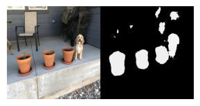
Let us visualize the results of this pretrained model
filepath = keras.utils.get_file(origin="https://i.imgur.com/gCNcJJI.jpg")
image = keras.utils.load_img(filepath)

resize = keras_cv.layers.Resizing(height=512, width=512)
image = resize(image)
image = keras.ops.expand_dims(np.array(image), axis=0)
preds = ops.expand_dims(ops.argmax(model(image), axis=-1), axis=-1)
keras_cv.visualization.plot_segmentation_mask_gallery(
    image,
    value_range=(0, 255),
    num_classes=1,
    y_true=None,
    y_pred=preds,
    scale=3,
    rows=1,
    cols=1,
)
Train a custom semantic segmentation model
In this guide, we’ll assemble a full training pipeline for a KerasCV DeepLabV3 semantic segmentation model. This includes data loading, augmentation, training, metric evaluation, and inference!
Download the data
We download Pascal VOC dataset with KerasCV datasets and split them into train dataset train_ds and eval_ds.
train_ds = load_voc(split="sbd_train")
eval_ds = load_voc(split="sbd_eval")
Preprocess the data
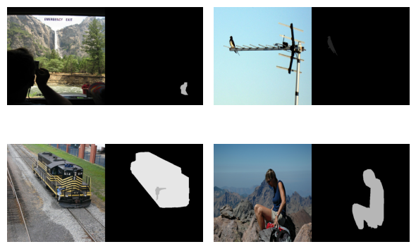
The preprocess_tfds_inputs utility function preprocesses the inputs to a dictionary of images and segmentation_masks. The images and segmentation masks are resized to 512x512. The resulting dataset is then batched into groups of 4 image and segmentation mask pairs.
A batch of this preprocessed input training data can be visualized using the keras_cv.visualization.plot_segmentation_mask_gallery function. This function takes a batch of images and segmentation masks as input and displays them in a grid.
def preprocess_tfds_inputs(inputs):
    def unpackage_tfds_inputs(tfds_inputs):
        return {
            "images": tfds_inputs["image"],
            "segmentation_masks": tfds_inputs["class_segmentation"],
        }

    outputs = inputs.map(unpackage_tfds_inputs)
    outputs = outputs.map(keras_cv.layers.Resizing(height=512, width=512))
    outputs = outputs.batch(4, drop_remainder=True)
    return outputs


train_ds = preprocess_tfds_inputs(train_ds)
batch = train_ds.take(1).get_single_element()
keras_cv.visualization.plot_segmentation_mask_gallery(
    batch["images"],
    value_range=(0, 255),
    num_classes=21,  # The number of classes for the oxford iiit pet dataset. The VOC dataset also includes 1 class for the background.
    y_true=batch["segmentation_masks"],
    scale=3,
    rows=2,
    cols=2,
)
The preprocessing is applied to the evaluation dataset eval_ds.
eval_ds = preprocess_tfds_inputs(eval_ds)Data Augmentation
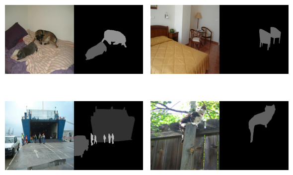
KerasCV provides a variety of image augmentation options. In this example, we will use the RandomFlip augmentation to augment the training dataset. The RandomFlip augmentation randomly flips the images in the training dataset horizontally or vertically. This can help to improve the model’s robustness to changes in the orientation of the objects in the images.
train_ds = train_ds.map(keras_cv.layers.RandomFlip())
batch = train_ds.take(1).get_single_element()

keras_cv.visualization.plot_segmentation_mask_gallery(
    batch["images"],
    value_range=(0, 255),
    num_classes=21,
    y_true=batch["segmentation_masks"],
    scale=3,
    rows=2,
    cols=2,
)
Model Configuration
Please feel free to modify the configurations for model training and note how the training results changes. This is an great exercise to get a better understanding of the training pipeline.
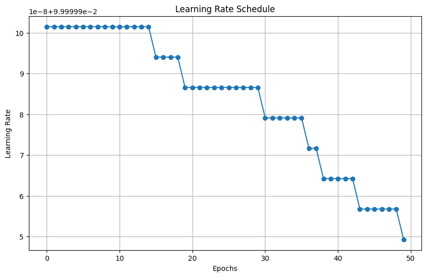
The learning rate schedule is used by the optimizer to calculate the learning rate for each epoch. The optimizer then uses the learning rate to update the weights of the model. In this case, the learning rate schedule uses a cosine decay function. A cosine decay function starts high and then decreases over time, eventually reaching zero. The cardinality of the VOC dataset is 2124 with a batch size of 4. The dataset cardinality is important for learning rate decay because it determines how many steps the model will train for. The initial learning rate is proportional to 0.007 and the decay steps are 2124. This means that the learning rate will start at INITIAL_LR and then decrease to zero over 2124 steps.
BATCH_SIZE = 4
INITIAL_LR = 0.007 * BATCH_SIZE / 16
EPOCHS = 1
NUM_CLASSES = 21
learning_rate = keras.optimizers.schedules.CosineDecay(
    INITIAL_LR,
    decay_steps=EPOCHS * 2124,
)
We instantiate a DeepLabV3+ model with a ResNet50 backbone pretrained on ImageNet classification: resnet50_v2_imagenet pre-trained weights will be used as the backbone feature extractor for the DeepLabV3Plus model. The num_classes parameter specifies the number of classes that the model will be trained to segment.
model = keras_cv.models.DeepLabV3Plus.from_preset(
    "resnet50_v2_imagenet", num_classes=NUM_CLASSES
)
Result
Downloading data from https://storage.googleapis.com/keras-cv/models/resnet50v2/imagenet/classification-v2-notop.h5
 94687928/94687928 ━━━━━━━━━━━━━━━━━━━━ 1s 0us/step
Compile the model
The model.compile() function sets up the training process for the model. It defines the - optimization algorithm - Stochastic Gradient Descent (SGD) - the loss function - categorical cross-entropy - the evaluation metrics - Mean IoU and categorical accuracy
Semantic segmentation evaluation metrics:
Mean Intersection over Union (MeanIoU): MeanIoU measures how well a semantic segmentation model accurately identifies and delineates different objects or regions in an image. It calculates the overlap between predicted and actual object boundaries, providing a score between 0 and 1, where 1 represents a perfect match.
Categorical Accuracy: Categorical Accuracy measures the proportion of correctly classified pixels in an image. It gives a simple percentage indicating how accurately the model predicts the categories of pixels in the entire image.
In essence, MeanIoU emphasizes the accuracy of identifying specific object boundaries, while Categorical Accuracy gives a broad overview of overall pixel-level correctness.
model.compile(
    optimizer=keras.optimizers.SGD(
        learning_rate=learning_rate, weight_decay=0.0001, momentum=0.9, clipnorm=10.0
    ),
    loss=keras.losses.CategoricalCrossentropy(from_logits=False),
    metrics=[
        keras.metrics.MeanIoU(
            num_classes=NUM_CLASSES, sparse_y_true=False, sparse_y_pred=False
        ),
        keras.metrics.CategoricalAccuracy(),
    ],
)

model.summary()
Result
Model: "deep_lab_v3_plus_1"
┏━━━━━━━━━━━━━━━━━━━━━┳━━━━━━━━━━━━━━━━━━━┳━━━━━━━━━┳━━━━━━━━━━━━━━━━━━━━━━┓
┃ Layer (type)        ┃ Output Shape      ┃ Param # ┃ Connected to         ┃
┡━━━━━━━━━━━━━━━━━━━━━╇━━━━━━━━━━━━━━━━━━━╇━━━━━━━━━╇━━━━━━━━━━━━━━━━━━━━━━┩
│ input_layer_9       │ (None, None,      │       0 │ -                    │
│ (InputLayer)        │ None, 3)          │         │                      │
├─────────────────────┼───────────────────┼─────────┼──────────────────────┤
│ functional_11       │ [(None, None,     │ 23,556… │ input_layer_9[0][0]  │
│ (Functional)        │ None, 256),       │         │                      │
│                     │ (None, None,      │         │                      │
│                     │ None, 2048)]      │         │                      │
├─────────────────────┼───────────────────┼─────────┼──────────────────────┤
│ spatial_pyramid_po… │ (None, None,      │ 15,538… │ functional_11[0][1]  │
│ (SpatialPyramidPoo… │ None, 256)        │         │                      │
├─────────────────────┼───────────────────┼─────────┼──────────────────────┤
│ encoder_output_ups… │ (None, None,      │       0 │ spatial_pyramid_poo… │
│ (UpSampling2D)      │ None, 256)        │         │                      │
├─────────────────────┼───────────────────┼─────────┼──────────────────────┤
│ sequential_14       │ (None, None,      │  12,480 │ functional_11[0][0]  │
│ (Sequential)        │ None, 48)         │         │                      │
├─────────────────────┼───────────────────┼─────────┼──────────────────────┤
│ concatenate_1       │ (None, None,      │       0 │ encoder_output_upsa… │
│ (Concatenate)       │ None, 304)        │         │ sequential_14[0][0]  │
├─────────────────────┼───────────────────┼─────────┼──────────────────────┤
│ sequential_15       │ (None, None,      │  84,224 │ concatenate_1[0][0]  │
│ (Sequential)        │ None, 21)         │         │                      │
└─────────────────────┴───────────────────┴─────────┴──────────────────────┘
 Total params: 39,191,488 (149.50 MB)
 Trainable params: 39,146,464 (149.33 MB)
 Non-trainable params: 45,024 (175.88 KB)
The utility function dict_to_tuple effectively transforms the dictionaries of training and validation datasets into tuples of images and one-hot encoded segmentation masks, which is used during training and evaluation of the DeepLabv3+ model.
def dict_to_tuple(x):
    import tensorflow as tf

    return x["images"], tf.one_hot(
        tf.cast(tf.squeeze(x["segmentation_masks"], axis=-1), "int32"), 21
    )


train_ds = train_ds.map(dict_to_tuple)
eval_ds = eval_ds.map(dict_to_tuple)

model.fit(train_ds, validation_data=eval_ds, epochs=EPOCHS)
Result
   2124/Unknown  735s 319ms/step - categorical_accuracy: 0.7026 - loss: 1.2143 - mean_io_u: 0.0706

/usr/lib/python3.10/contextlib.py:153: UserWarning: Your input ran out of data; interrupting training. Make sure that your dataset or generator can generate at least `steps_per_epoch * epochs` batches. You may need to use the `.repeat()` function when building your dataset.
  self.gen.throw(typ, value, traceback)

 2124/2124 ━━━━━━━━━━━━━━━━━━━━ 813s 356ms/step - categorical_accuracy: 0.7026 - loss: 1.2143 - mean_io_u: 0.0706 - val_categorical_accuracy: 0.7768 - val_loss: 0.8223 - val_mean_io_u: 0.1593

<keras.src.callbacks.history.History at 0x7f261a534640>
Predictions with trained model
Now that the model training of DeepLabv3+ has completed, let’s test it by making predications on a few sample images.
test_ds = load_voc(split="sbd_eval")
test_ds = preprocess_tfds_inputs(test_ds)

images, masks = next(iter(train_ds.take(1)))
images = ops.convert_to_tensor(images)
masks = ops.convert_to_tensor(masks)
preds = ops.expand_dims(ops.argmax(model(images), axis=-1), axis=-1)
masks = ops.expand_dims(ops.argmax(masks, axis=-1), axis=-1)

keras_cv.visualization.plot_segmentation_mask_gallery(
    images,
    value_range=(0, 255),
    num_classes=21,
    y_true=masks,
    y_pred=preds,
    scale=3,
    rows=1,
    cols=4,
)
Here are some additional tips for using the KerasCV DeepLabv3+ model:
- The model can be trained on a variety of datasets, including the COCO dataset, the PASCAL VOC dataset, and the Cityscapes dataset.
- The model can be fine-tuned on a custom dataset to improve its performance on a specific task.
- The model can be used to perform real-time inference on images.
- Also, try out KerasCV’s SegFormer model
keras_cv.models.segmentation.SegFormer. The SegFormer model is a newer model that has been shown to achieve state-of-the-art results on a variety of image segmentation benchmarks. It is based on the Swin Transformer architecture, and it is more efficient and accurate than previous image segmentation models.