Object Detection with KerasCV
- Original Link : https://keras.io/guides/keras_cv/object_detection_keras_cv/
- Last Checked at : 2024-11-19
Author: lukewood, Ian Stenbit, Tirth Patel
Date created: 2023/04/08
Last modified: 2023/08/10
Description: Train an object detection model with KerasCV.
KerasCV offers a complete set of production grade APIs to solve object detection problems. These APIs include object-detection-specific data augmentation techniques, Keras native COCO metrics, bounding box format conversion utilities, visualization tools, pretrained object detection models, and everything you need to train your own state of the art object detection models!
Let’s give KerasCV’s object detection API a spin.
!pip install -q --upgrade keras-cv
!pip install -q --upgrade keras  # Upgrade to Keras 3.
import os
os.environ["KERAS_BACKEND"] = "jax" # @param ["tensorflow", "jax", "torch"]
from tensorflow import data as tf_data
import tensorflow_datasets as tfds
import keras
import keras_cv
import numpy as np
from keras_cv import bounding_box
import os
from keras_cv import visualization
import tqdmObject detection introduction
Object detection is the process of identifying, classifying, and localizing objects within a given image. Typically, your inputs are images, and your labels are bounding boxes with optional class labels. Object detection can be thought of as an extension of classification, however instead of one class label for the image, you must detect and localize an arbitrary number of classes.
For example:
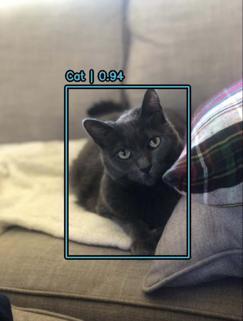
The data for the above image may look something like this:
image = [height, width, 3]
bounding_boxes = {
  "classes": [0], # 0 is an arbitrary class ID representing "cat"
  "boxes": [[0.25, 0.4, .15, .1]]
   # bounding box is in "rel_xywh" format
   # so 0.25 represents the start of the bounding box 25% of
   # the way across the image.
   # The .15 represents that the width is 15% of the image width.
}
Since the inception of You Only Look Once (aka YOLO), object detection has primarily been solved using deep learning. Most deep learning architectures do this by cleverly framing the object detection problem as a combination of many small classification problems and many regression problems.
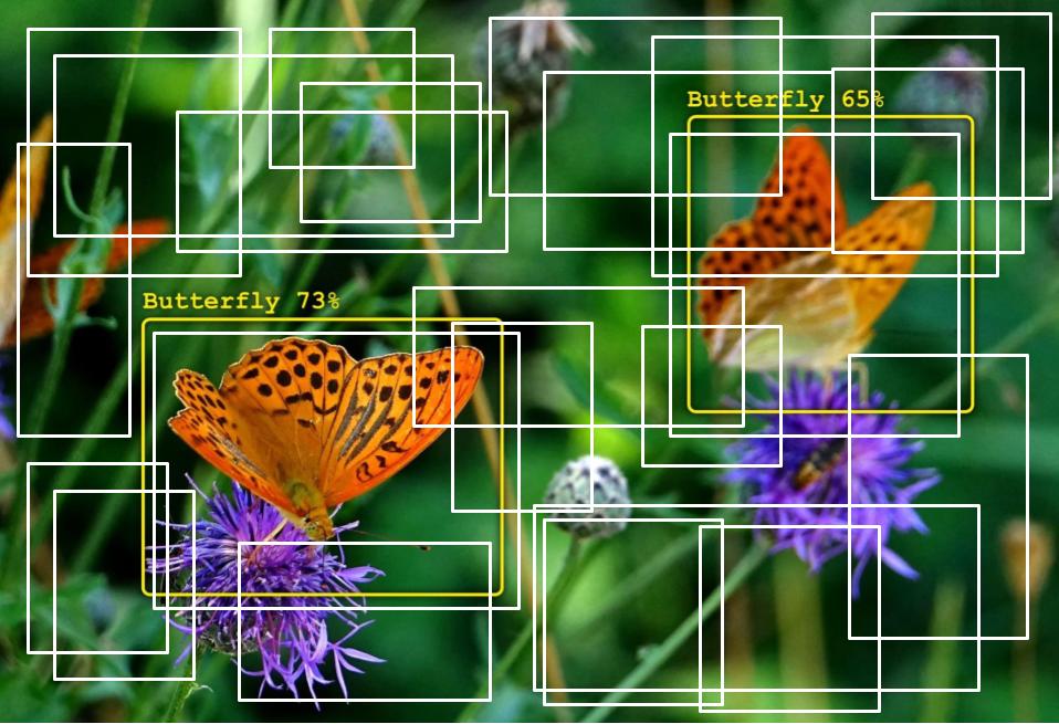
More specifically, this is done by generating many anchor boxes of varying shapes and sizes across the input images and assigning them each a class label, as well as x, y, width and height offsets. The model is trained to predict the class labels of each box, as well as the x, y, width, and height offsets of each box that is predicted to be an object.
Visualization of some sample anchor boxes:
Objection detection is a technically complex problem but luckily we offer a bulletproof approach to getting great results. Let’s do this!
Perform detections with a pretrained model

The highest level API in the KerasCV Object Detection API is the keras_cv.models API. This API includes fully pretrained object detection models, such as keras_cv.models.YOLOV8Detector.
Let’s get started by constructing a YOLOV8Detector pretrained on the pascalvoc dataset.
pretrained_model = keras_cv.models.YOLOV8Detector.from_preset(
    "yolo_v8_m_pascalvoc", bounding_box_format="xywh"
)
Notice the bounding_box_format argument?
Recall in the section above, the format of bounding boxes:
bounding_boxes = {
  "classes": [num_boxes],
  "boxes": [num_boxes, 4]
}
This argument describes exactly what format the values in the "boxes" field of the label dictionary take in your pipeline. For example, a box in xywh format with its top left corner at the coordinates (100, 100) with a width of 55 and a height of 70 would be represented by:
[100, 100, 55, 75]or equivalently in xyxy format:
[100, 100, 155, 175]While this may seem simple, it is a critical piece of the KerasCV object detection API! Every component that processes bounding boxes requires a bounding_box_format argument. You can read more about KerasCV bounding box formats in the API docs.
This is done because there is no one correct format for bounding boxes! Components in different pipelines expect different formats, and so by requiring them to be specified we ensure that our components remain readable, reusable, and clear. Box format conversion bugs are perhaps the most common bug surface in object detection pipelines - by requiring this parameter we mitigate against these bugs (especially when combining code from many sources).
Next let’s load an image:
filepath = keras.utils.get_file(origin="https://i.imgur.com/gCNcJJI.jpg")
image = keras.utils.load_img(filepath)
image = np.array(image)

visualization.plot_image_gallery(
    np.array([image]),
    value_range=(0, 255),
    rows=1,
    cols=1,
    scale=5,
)
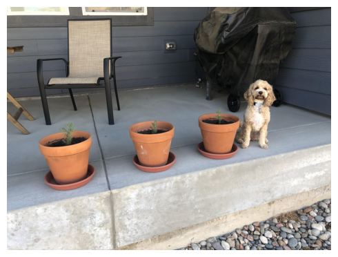
To use the YOLOV8Detector architecture with a ResNet50 backbone, you’ll need to resize your image to a size that is divisible by 64. This is to ensure compatibility with the number of downscaling operations done by the convolution layers in the ResNet.
If the resize operation distorts the input’s aspect ratio, the model will perform signficantly poorer. For the pretrained "yolo_v8_m_pascalvoc" preset we are using, the final MeanAveragePrecision on the pascalvoc/2012 evaluation set drops to 0.15 from 0.38 when using a naive resizing operation.
Additionally, if you crop to preserve the aspect ratio as you do in classification your model may entirely miss some bounding boxes. As such, when running inference on an object detection model we recommend the use of padding to the desired size, while resizing the longest size to match the aspect ratio.
KerasCV makes resizing properly easy; simply pass pad_to_aspect_ratio=True to a keras_cv.layers.Resizing layer.
This can be implemented in one line of code:
inference_resizing = keras_cv.layers.Resizing(
    640, 640, pad_to_aspect_ratio=True, bounding_box_format="xywh"
)
This can be used as our inference preprocessing pipeline:
image_batch = inference_resizing([image])keras_cv.visualization.plot_bounding_box_gallery() supports a class_mapping parameter to highlight what class each box was assigned to. Let’s assemble a class mapping now.
class_ids = [
    "Aeroplane",
    "Bicycle",
    "Bird",
    "Boat",
    "Bottle",
    "Bus",
    "Car",
    "Cat",
    "Chair",
    "Cow",
    "Dining Table",
    "Dog",
    "Horse",
    "Motorbike",
    "Person",
    "Potted Plant",
    "Sheep",
    "Sofa",
    "Train",
    "Tvmonitor",
    "Total",
]
class_mapping = dict(zip(range(len(class_ids)), class_ids))
Just like any other keras.Model you can predict bounding boxes using the model.predict() API.
y_pred = pretrained_model.predict(image_batch)
# y_pred is a bounding box Tensor:
# {"classes": ..., boxes": ...}
visualization.plot_bounding_box_gallery(
    image_batch,
    value_range=(0, 255),
    rows=1,
    cols=1,
    y_pred=y_pred,
    scale=5,
    font_scale=0.7,
    bounding_box_format="xywh",
    class_mapping=class_mapping,
)
Result
1/1 ━━━━━━━━━━━━━━━━━━━━ 11s 11s/step
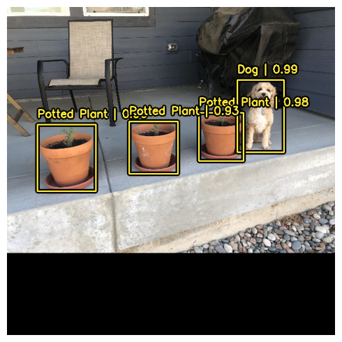
In order to support this easy and intuitive inference workflow, KerasCV performs non-max suppression inside of the YOLOV8Detector class. Non-max suppression is a traditional computing algorithm that solves the problem of a model detecting multiple boxes for the same object.
Non-max suppression is a highly configurable algorithm, and in most cases you will want to customize the settings of your model’s non-max suppression operation. This can be done by overriding to the prediction_decoder argument.
To show this concept off, let’s temporarily disable non-max suppression on our YOLOV8Detector. This can be done by writing to the prediction_decoder attribute.
# The following NonMaxSuppression layer is equivalent to disabling the operation
prediction_decoder = keras_cv.layers.NonMaxSuppression(
    bounding_box_format="xywh",
    from_logits=True,
    iou_threshold=1.0,
    confidence_threshold=0.0,
)
pretrained_model = keras_cv.models.YOLOV8Detector.from_preset(
    "yolo_v8_m_pascalvoc",
    bounding_box_format="xywh",
    prediction_decoder=prediction_decoder,
)

y_pred = pretrained_model.predict(image_batch)
visualization.plot_bounding_box_gallery(
    image_batch,
    value_range=(0, 255),
    rows=1,
    cols=1,
    y_pred=y_pred,
    scale=5,
    font_scale=0.7,
    bounding_box_format="xywh",
    class_mapping=class_mapping,
)
Result
1/1 ━━━━━━━━━━━━━━━━━━━━ 5s 5s/step
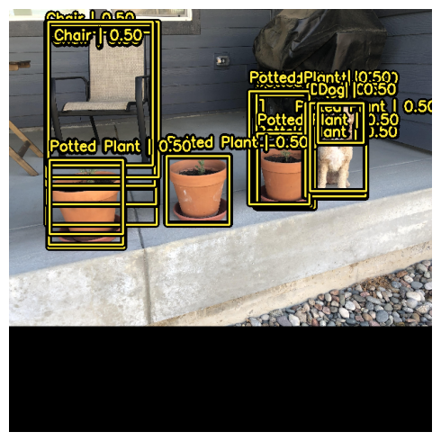
Next, let’s re-configure keras_cv.layers.NonMaxSuppression for our use case! In this case, we will tune the iou_threshold to 0.2, and the confidence_threshold to 0.7.
Raising the confidence_threshold will cause the model to only output boxes that have a higher confidence score. iou_threshold controls the threshold of intersection over union (IoU) that two boxes must have in order for one to be pruned out. More information on these parameters may be found in the TensorFlow API docs
prediction_decoder = keras_cv.layers.NonMaxSuppression(
    bounding_box_format="xywh",
    from_logits=True,
    # Decrease the required threshold to make predictions get pruned out
    iou_threshold=0.2,
    # Tune confidence threshold for predictions to pass NMS
    confidence_threshold=0.7,
)
pretrained_model = keras_cv.models.YOLOV8Detector.from_preset(
    "yolo_v8_m_pascalvoc",
    bounding_box_format="xywh",
    prediction_decoder=prediction_decoder,
)

y_pred = pretrained_model.predict(image_batch)
visualization.plot_bounding_box_gallery(
    image_batch,
    value_range=(0, 255),
    rows=1,
    cols=1,
    y_pred=y_pred,
    scale=5,
    font_scale=0.7,
    bounding_box_format="xywh",
    class_mapping=class_mapping,
)
Result
1/1 ━━━━━━━━━━━━━━━━━━━━ 5s 5s/step

That looks a lot better!
Train a custom object detection model

Whether you’re an object detection amateur or a well seasoned veteran, assembling an object detection pipeline from scratch is a massive undertaking. Luckily, all KerasCV object detection APIs are built as modular components. Whether you need a complete pipeline, just an object detection model, or even just a conversion utility to transform your boxes from xywh format to xyxy, KerasCV has you covered.
In this guide, we’ll assemble a full training pipeline for a KerasCV object detection model. This includes data loading, augmentation, metric evaluation, and inference!
To get started, let’s sort out all of our imports and define global configuration parameters.
BATCH_SIZE = 4Data loading
To get started, let’s discuss data loading and bounding box formatting. KerasCV has a predefined format for bounding boxes. To comply with this, you should package your bounding boxes into a dictionary matching the specification below:
bounding_boxes = {
    # num_boxes may be a Ragged dimension
    'boxes': Tensor(shape=[batch, num_boxes, 4]),
    'classes': Tensor(shape=[batch, num_boxes])
}
bounding_boxes['boxes'] contains the coordinates of your bounding box in a KerasCV supported bounding_box_format. KerasCV requires a bounding_box_format argument in all components that process bounding boxes. This is done to maximize your ability to plug and play individual components into their object detection pipelines, as well as to make code self-documenting across object detection pipelines.
To match the KerasCV API style, it is recommended that when writing a custom data loader, you also support a bounding_box_format argument. This makes it clear to those invoking your data loader what format the bounding boxes are in. In this example, we format our boxes to xywh format.
For example:
train_ds, ds_info = your_data_loader.load(
    split='train', bounding_box_format='xywh', batch_size=8
)
This clearly yields bounding boxes in the format xywh. You can read more about KerasCV bounding box formats in the API docs.
Our data comes loaded into the format {"images": images, "bounding_boxes": bounding_boxes}. This format is supported in all KerasCV preprocessing components.
Let’s load some data and verify that the data looks as we expect it to.
def visualize_dataset(inputs, value_range, rows, cols, bounding_box_format):
    inputs = next(iter(inputs.take(1)))
    images, bounding_boxes = inputs["images"], inputs["bounding_boxes"]
    visualization.plot_bounding_box_gallery(
        images,
        value_range=value_range,
        rows=rows,
        cols=cols,
        y_true=bounding_boxes,
        scale=5,
        font_scale=0.7,
        bounding_box_format=bounding_box_format,
        class_mapping=class_mapping,
    )


def unpackage_raw_tfds_inputs(inputs, bounding_box_format):
    image = inputs["image"]
    boxes = keras_cv.bounding_box.convert_format(
        inputs["objects"]["bbox"],
        images=image,
        source="rel_yxyx",
        target=bounding_box_format,
    )
    bounding_boxes = {
        "classes": inputs["objects"]["label"],
        "boxes": boxes,
    }
    return {"images": image, "bounding_boxes": bounding_boxes}


def load_pascal_voc(split, dataset, bounding_box_format):
    ds = tfds.load(dataset, split=split, with_info=False, shuffle_files=True)
    ds = ds.map(
        lambda x: unpackage_raw_tfds_inputs(x, bounding_box_format=bounding_box_format),
        num_parallel_calls=tf_data.AUTOTUNE,
    )
    return ds


train_ds = load_pascal_voc(
    split="train", dataset="voc/2007", bounding_box_format="xywh"
)
eval_ds = load_pascal_voc(split="test", dataset="voc/2007", bounding_box_format="xywh")

train_ds = train_ds.shuffle(BATCH_SIZE * 4)
Next, let’s batch our data.
In KerasCV object detection tasks it is recommended that users use ragged batches of inputs. This is due to the fact that images may be of different sizes in PascalVOC, as well as the fact that there may be different numbers of bounding boxes per image.
To construct a ragged dataset in a tf.data pipeline, you can use the ragged_batch() method.
train_ds = train_ds.ragged_batch(BATCH_SIZE, drop_remainder=True)
eval_ds = eval_ds.ragged_batch(BATCH_SIZE, drop_remainder=True)
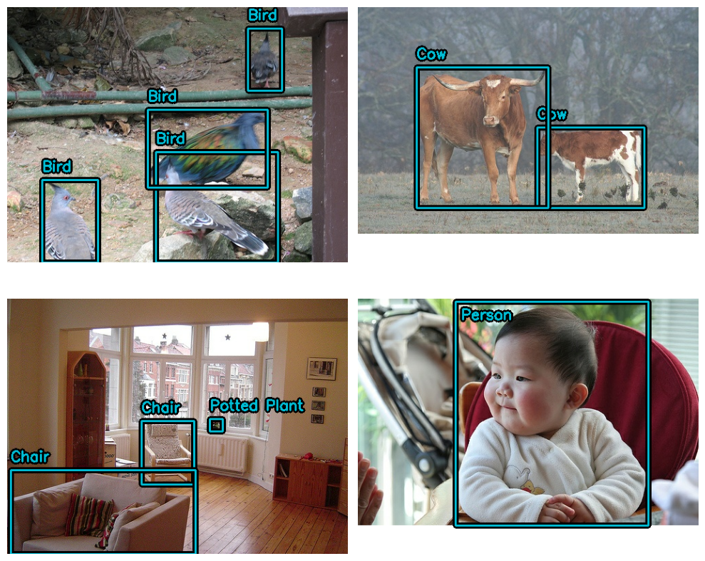
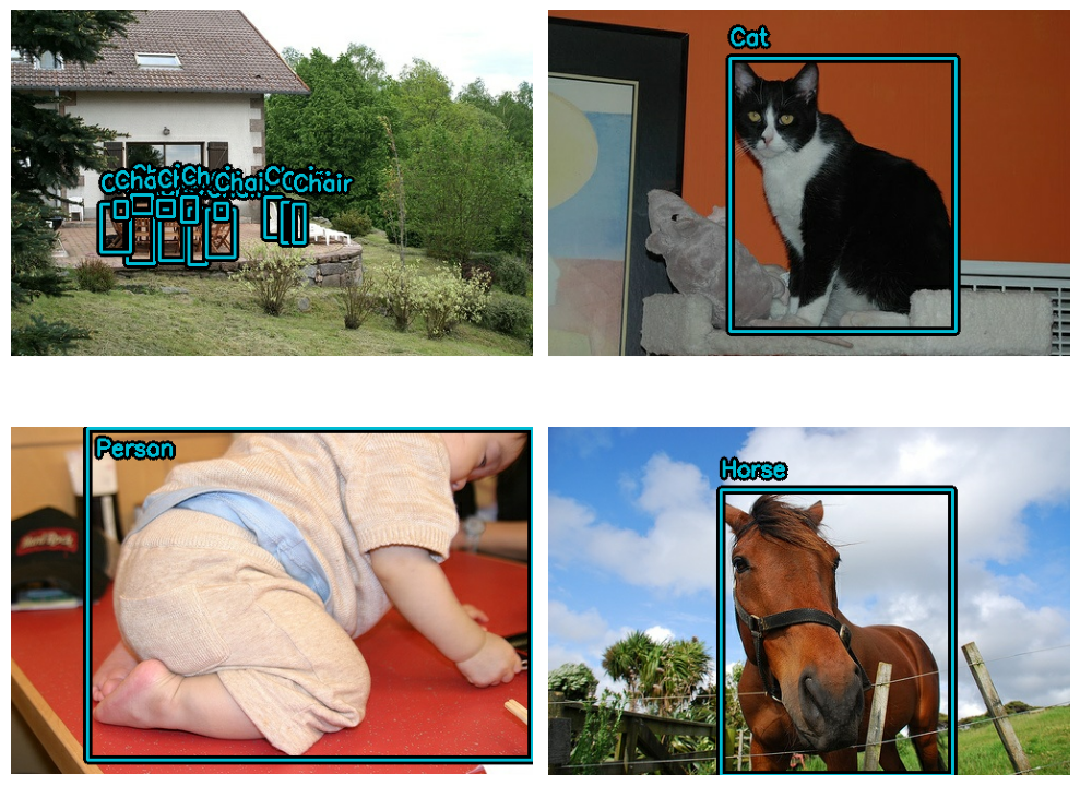
Let’s make sure our dataset is following the format KerasCV expects. By using the visualize_dataset() function, you can visually verify that your data is in the format that KerasCV expects. If the bounding boxes are not visible or are visible in the wrong locations that is a sign that your data is mis-formatted.
visualize_dataset(
    train_ds, bounding_box_format="xywh", value_range=(0, 255), rows=2, cols=2
)
And for the eval set:
visualize_dataset(
    eval_ds,
    bounding_box_format="xywh",
    value_range=(0, 255),
    rows=2,
    cols=2,
    # If you are not running your experiment on a local machine, you can also
    # make `visualize_dataset()` dump the plot to a file using `path`:
    # path="eval.png"
)
Looks like everything is structured as expected. Now we can move on to constructing our data augmentation pipeline.
Data augmentation
One of the most challenging tasks when constructing object detection pipelines is data augmentation. Image augmentation techniques must be aware of the underlying bounding boxes, and must update them accordingly.
Luckily, KerasCV natively supports bounding box augmentation with its extensive library of data augmentation layers. The code below loads the Pascal VOC dataset, and performs on-the-fly, bounding-box-friendly data augmentation inside a tf.data pipeline.
augmenters = [
    keras_cv.layers.RandomFlip(mode="horizontal", bounding_box_format="xywh"),
    keras_cv.layers.JitteredResize(
        target_size=(640, 640), scale_factor=(0.75, 1.3), bounding_box_format="xywh"
    ),
]


def create_augmenter_fn(augmenters):
    def augmenter_fn(inputs):
        for augmenter in augmenters:
            inputs = augmenter(inputs)
        return inputs

    return augmenter_fn


augmenter_fn = create_augmenter_fn(augmenters)

train_ds = train_ds.map(augmenter_fn, num_parallel_calls=tf_data.AUTOTUNE)
visualize_dataset(
    train_ds, bounding_box_format="xywh", value_range=(0, 255), rows=2, cols=2
)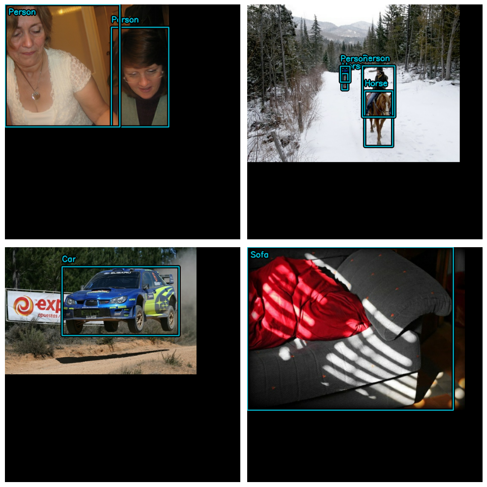
Great! We now have a bounding-box-friendly data augmentation pipeline. Let’s format our evaluation dataset to match. Instead of using JitteredResize, let’s use the deterministic keras_cv.layers.Resizing() layer.
inference_resizing = keras_cv.layers.Resizing(
    640, 640, bounding_box_format="xywh", pad_to_aspect_ratio=True
)
eval_ds = eval_ds.map(inference_resizing, num_parallel_calls=tf_data.AUTOTUNE)
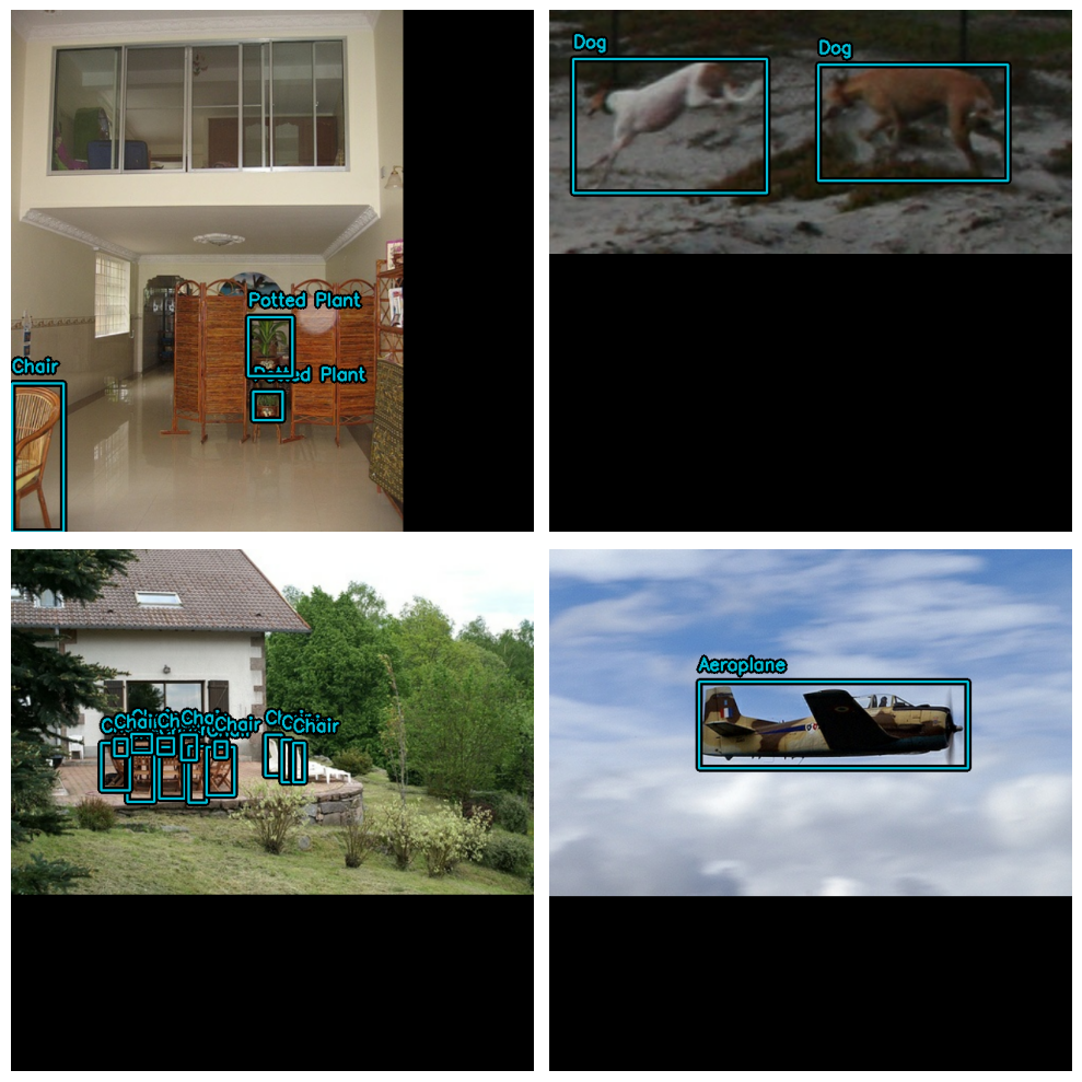
Due to the fact that the resize operation differs between the train dataset, which uses JitteredResize() to resize images, and the inference dataset, which uses layers.Resizing(pad_to_aspect_ratio=True), it is good practice to visualize both datasets:
visualize_dataset(
    eval_ds, bounding_box_format="xywh", value_range=(0, 255), rows=2, cols=2
)
Finally, let’s unpackage our inputs from the preprocessing dictionary, and prepare to feed the inputs into our model. In order to be TPU compatible, bounding box Tensors need to be Dense instead of Ragged.
def dict_to_tuple(inputs):
    return inputs["images"], bounding_box.to_dense(
        inputs["bounding_boxes"], max_boxes=32
    )


train_ds = train_ds.map(dict_to_tuple, num_parallel_calls=tf_data.AUTOTUNE)
eval_ds = eval_ds.map(dict_to_tuple, num_parallel_calls=tf_data.AUTOTUNE)

train_ds = train_ds.prefetch(tf_data.AUTOTUNE)
eval_ds = eval_ds.prefetch(tf_data.AUTOTUNE)
Optimizer
In this guide, we use a standard SGD optimizer and rely on the keras.callbacks.ReduceLROnPlateau callback to reduce the learning rate.
You will always want to include a global_clipnorm when training object detection models. This is to remedy exploding gradient problems that frequently occur when training object detection models.
base_lr = 0.005
# including a global_clipnorm is extremely important in object detection tasks
optimizer = keras.optimizers.SGD(
    learning_rate=base_lr, momentum=0.9, global_clipnorm=10.0
)
To achieve the best results on your dataset, you’ll likely want to hand craft a PiecewiseConstantDecay learning rate schedule. While PiecewiseConstantDecay schedules tend to perform better, they don’t translate between problems.
Loss functions
You may not be familiar with the "ciou" loss. While not common in other models, this loss is sometimes used in the object detection world.
In short, “Complete IoU” is a flavour of the Intersection over Union loss and is used due to its convergence properties.
In KerasCV, you can use this loss simply by passing the string "ciou" to compile(). We also use standard binary crossentropy loss for the class head.
pretrained_model.compile(
    classification_loss="binary_crossentropy",
    box_loss="ciou",
)
Metric evaluation
The most popular object detection metrics are COCO metrics, which were published alongside the MSCOCO dataset. KerasCV provides an easy-to-use suite of COCO metrics under the keras_cv.callbacks.PyCOCOCallback symbol. Note that we use a Keras callback instead of a Keras metric to compute COCO metrics. This is because computing COCO metrics requires storing all of a model’s predictions for the entire evaluation dataset in memory at once, which is impractical to do during training time.
coco_metrics_callback = keras_cv.callbacks.PyCOCOCallback(
    eval_ds.take(20), bounding_box_format="xywh"
)
Our data pipeline is now complete! We can now move on to model creation and training.
Model creation
Next, let’s use the KerasCV API to construct an untrained YOLOV8Detector model. In this tutorial we use a pretrained ResNet50 backbone from the imagenet dataset.
KerasCV makes it easy to construct a YOLOV8Detector with any of the KerasCV backbones. Simply use one of the presets for the architecture you’d like!
For example:
model = keras_cv.models.YOLOV8Detector.from_preset(
    "resnet50_imagenet",
    # For more info on supported bounding box formats, visit
    # https://keras.io/api/keras_cv/bounding_box/
    bounding_box_format="xywh",
    num_classes=20,
)
That is all it takes to construct a KerasCV YOLOv8. The YOLOv8 accepts tuples of dense image Tensors and bounding box dictionaries to fit() and train_on_batch()
This matches what we have constructed in our input pipeline above.
Training our model
All that is left to do is train our model. KerasCV object detection models follow the standard Keras workflow, leveraging compile() and fit().
Let’s compile our model:
model.compile(
    classification_loss="binary_crossentropy",
    box_loss="ciou",
    optimizer=optimizer,
)
If you want to fully train the model, remove .take(20) from all dataset references (below and in the initialization of the metrics callback).
model.fit(
    train_ds.take(20),
    # Run for 10-35~ epochs to achieve good scores.
    epochs=1,
    callbacks=[coco_metrics_callback],
)
Result
 20/20 ━━━━━━━━━━━━━━━━━━━━ 7s 59ms/step
creating index...
index created!
creating index...
index created!
Running per image evaluation...
Evaluate annotation type *bbox*
DONE (t=0.16s).
Accumulating evaluation results...
DONE (t=0.07s).
 Average Precision  (AP) @[ IoU=0.50:0.95 | area=   all | maxDets=100 ] = 0.000
 Average Precision  (AP) @[ IoU=0.50      | area=   all | maxDets=100 ] = 0.000
 Average Precision  (AP) @[ IoU=0.75      | area=   all | maxDets=100 ] = 0.000
 Average Precision  (AP) @[ IoU=0.50:0.95 | area= small | maxDets=100 ] = 0.000
 Average Precision  (AP) @[ IoU=0.50:0.95 | area=medium | maxDets=100 ] = 0.000
 Average Precision  (AP) @[ IoU=0.50:0.95 | area= large | maxDets=100 ] = 0.000
 Average Recall     (AR) @[ IoU=0.50:0.95 | area=   all | maxDets=  1 ] = 0.002
 Average Recall     (AR) @[ IoU=0.50:0.95 | area=   all | maxDets= 10 ] = 0.002
 Average Recall     (AR) @[ IoU=0.50:0.95 | area=   all | maxDets=100 ] = 0.002
 Average Recall     (AR) @[ IoU=0.50:0.95 | area= small | maxDets=100 ] = 0.000
 Average Recall     (AR) @[ IoU=0.50:0.95 | area=medium | maxDets=100 ] = 0.000
 Average Recall     (AR) @[ IoU=0.50:0.95 | area= large | maxDets=100 ] = 0.002
 20/20 ━━━━━━━━━━━━━━━━━━━━ 73s 681ms/step - loss: 9221.7988 - val_AP: 3.1673e-05 - val_AP50: 2.1886e-04 - val_AP75: 0.0000e+00 - val_APs: 0.0000e+00 - val_APm: 0.0000e+00 - val_APl: 3.1673e-05 - val_ARmax1: 0.0016 - val_ARmax10: 0.0021 - val_ARmax100: 0.0021 - val_ARs: 0.0000e+00 - val_ARm: 0.0000e+00 - val_ARl: 0.0021

<keras.src.callbacks.history.History at 0x7fb23010a850>
Inference and plotting results
KerasCV makes object detection inference simple. model.predict(images) returns a tensor of bounding boxes. By default, YOLOV8Detector.predict() will perform a non max suppression operation for you.
In this section, we will use a keras_cv provided preset:
model = keras_cv.models.YOLOV8Detector.from_preset(
    "yolo_v8_m_pascalvoc", bounding_box_format="xywh"
)
Next, for convenience we construct a dataset with larger batches:
visualization_ds = eval_ds.unbatch()
visualization_ds = visualization_ds.ragged_batch(16)
visualization_ds = visualization_ds.shuffle(8)
Let’s create a simple function to plot our inferences:
def visualize_detections(model, dataset, bounding_box_format):
    images, y_true = next(iter(dataset.take(1)))
    y_pred = model.predict(images)
    visualization.plot_bounding_box_gallery(
        images,
        value_range=(0, 255),
        bounding_box_format=bounding_box_format,
        y_true=y_true,
        y_pred=y_pred,
        scale=4,
        rows=2,
        cols=2,
        show=True,
        font_scale=0.7,
        class_mapping=class_mapping,
    )
You may need to configure your NonMaxSuppression operation to achieve visually appealing results.
model.prediction_decoder = keras_cv.layers.NonMaxSuppression(
    bounding_box_format="xywh",
    from_logits=True,
    iou_threshold=0.5,
    confidence_threshold=0.75,
)

visualize_detections(model, dataset=visualization_ds, bounding_box_format="xywh")
Result
1/1 ━━━━━━━━━━━━━━━━━━━━ 16s 16s/step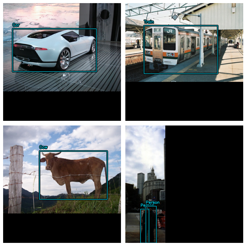
Awesome! One final helpful pattern to be aware of is to visualize detections in a keras.callbacks.Callback to monitor training:
class VisualizeDetections(keras.callbacks.Callback):
    def on_epoch_end(self, epoch, logs):
        visualize_detections(
            self.model, bounding_box_format="xywh", dataset=visualization_ds
        )
Takeaways and next steps
KerasCV makes it easy to construct state-of-the-art object detection pipelines. In this guide, we started off by writing a data loader using the KerasCV bounding box specification. Following this, we assembled a production grade data augmentation pipeline using KerasCV preprocessing layers in <50 lines of code.
KerasCV object detection components can be used independently, but also have deep integration with each other. KerasCV makes authoring production grade bounding box augmentation, model training, visualization, and metric evaluation easy.
Some follow up exercises for the reader:
- add additional augmentation techniques to improve model performance
- tune the hyperparameters and data augmentation used to produce high quality results
- train an object detection model on your own dataset
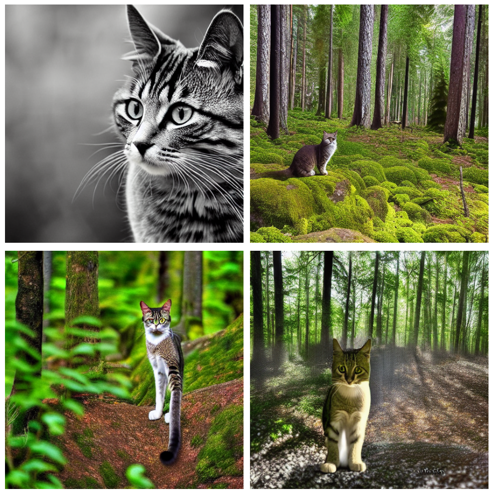
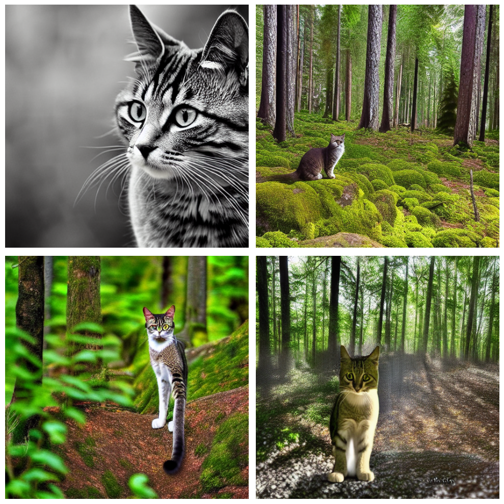
One last fun code snippet to showcase the power of KerasCV’s API!
stable_diffusion = keras_cv.models.StableDiffusionV2(512, 512)
images = stable_diffusion.text_to_image(
    prompt="A zoomed out photograph of a cool looking cat.  The cat stands in a beautiful forest",
    negative_prompt="unrealistic, bad looking, malformed",
    batch_size=4,
    seed=1231,
)
encoded_predictions = model(images)
y_pred = model.decode_predictions(encoded_predictions, images)
visualization.plot_bounding_box_gallery(
    images,
    value_range=(0, 255),
    y_pred=y_pred,
    rows=2,
    cols=2,
    scale=5,
    font_scale=0.7,
    bounding_box_format="xywh",
    class_mapping=class_mapping,
)
Result
By using this model checkpoint, you acknowledge that its usage is subject to the terms of the CreativeML Open RAIL++-M license at https://github.com/Stability-AI/stablediffusion/blob/main/LICENSE-MODEL
 50/50 ━━━━━━━━━━━━━━━━━━━━ 47s 356ms/step