CutMix, MixUp, and RandAugment image augmentation with KerasCV
- Original Link : https://keras.io/guides/keras_cv/cut_mix_mix_up_and_rand_augment/
- Last Checked at : 2024-11-19
Author: lukewood
Date created: 2022/04/08
Last modified: 2022/04/08
Description: Use KerasCV to augment images with CutMix, MixUp, RandAugment, and more.
Overview
KerasCV makes it easy to assemble state-of-the-art, industry-grade data augmentation pipelines for image classification and object detection tasks. KerasCV offers a wide suite of preprocessing layers implementing common data augmentation techniques.
Perhaps three of the most useful layers are keras_cv.layers.CutMix, keras_cv.layers.MixUp, and keras_cv.layers.RandAugment. These layers are used in nearly all state-of-the-art image classification pipelines.
This guide will show you how to compose these layers into your own data augmentation pipeline for image classification tasks. This guide will also walk you through the process of customizing a KerasCV data augmentation pipeline.
Imports & setup
KerasCV uses Keras 3 to work with any of TensorFlow, PyTorch or Jax. In the guide below, we will use the jax backend. This guide runs in TensorFlow or PyTorch backends with zero changes, simply update the KERAS_BACKEND below.
!pip install -q --upgrade keras-cv
!pip install -q --upgrade keras  # Upgrade to Keras 3.
We begin by importing all required packages:
import os

os.environ["KERAS_BACKEND"] = "jax"  # @param ["tensorflow", "jax", "torch"]

import matplotlib.pyplot as plt

# Import tensorflow for [`tf.data`](https://www.tensorflow.org/api_docs/python/tf/data) and its preprocessing map functions
import tensorflow as tf
import tensorflow_datasets as tfds
import keras
import keras_cv
Data loading
This guide uses the 102 Category Flower Dataset for demonstration purposes.
To get started, we first load the dataset:
BATCH_SIZE = 32
AUTOTUNE = tf.data.AUTOTUNE
tfds.disable_progress_bar()
data, dataset_info = tfds.load("oxford_flowers102", with_info=True, as_supervised=True)
train_steps_per_epoch = dataset_info.splits["train"].num_examples // BATCH_SIZE
val_steps_per_epoch = dataset_info.splits["test"].num_examples // BATCH_SIZE
Result
 Downloading and preparing dataset 328.90 MiB (download: 328.90 MiB, generated: 331.34 MiB, total: 660.25 MiB) to /usr/local/google/home/rameshsampath/tensorflow_datasets/oxford_flowers102/2.1.1...
 Dataset oxford_flowers102 downloaded and prepared to /usr/local/google/home/rameshsampath/tensorflow_datasets/oxford_flowers102/2.1.1. Subsequent calls will reuse this data.
Next, we resize the images to a constant size, (224, 224), and one-hot encode the labels. Please note that keras_cv.layers.CutMix and keras_cv.layers.MixUp expect targets to be one-hot encoded. This is because they modify the values of the targets in a way that is not possible with a sparse label representation.
IMAGE_SIZE = (224, 224)
num_classes = dataset_info.features["label"].num_classes


def to_dict(image, label):
    image = tf.image.resize(image, IMAGE_SIZE)
    image = tf.cast(image, tf.float32)
    label = tf.one_hot(label, num_classes)
    return {"images": image, "labels": label}


def prepare_dataset(dataset, split):
    if split == "train":
        return (
            dataset.shuffle(10 * BATCH_SIZE)
            .map(to_dict, num_parallel_calls=AUTOTUNE)
            .batch(BATCH_SIZE)
        )
    if split == "test":
        return dataset.map(to_dict, num_parallel_calls=AUTOTUNE).batch(BATCH_SIZE)


def load_dataset(split="train"):
    dataset = data[split]
    return prepare_dataset(dataset, split)


train_dataset = load_dataset()
Let’s inspect some samples from our dataset:
def visualize_dataset(dataset, title):
    plt.figure(figsize=(6, 6)).suptitle(title, fontsize=18)
    for i, samples in enumerate(iter(dataset.take(9))):
        images = samples["images"]
        plt.subplot(3, 3, i + 1)
        plt.imshow(images[0].numpy().astype("uint8"))
        plt.axis("off")
    plt.show()


visualize_dataset(train_dataset, title="Before Augmentation")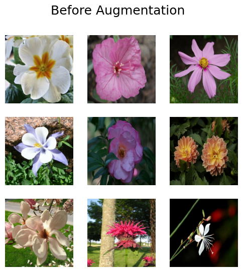
Great! Now we can move onto the augmentation step.
RandAugment
RandAugment has been shown to provide improved image classification results across numerous datasets. It performs a standard set of augmentations on an image.
To use RandAugment in KerasCV, you need to provide a few values:
value_rangedescribes the range of values covered in your imagesmagnitudeis a value between 0 and 1, describing the strength of the perturbations appliedaugmentations_per_imageis an integer telling the layer how many augmentations to apply to each individual image- (Optional)
magnitude_stddevallowsmagnitudeto be randomly sampled from a distribution with a standard deviation ofmagnitude_stddev - (Optional)
rateindicates the probability to apply the augmentation applied at each layer.
You can read more about these parameters in the RandAugment API documentation.
Let’s use KerasCV’s RandAugment implementation.
rand_augment = keras_cv.layers.RandAugment(
    value_range=(0, 255),
    augmentations_per_image=3,
    magnitude=0.3,
    magnitude_stddev=0.2,
    rate=1.0,
)


def apply_rand_augment(inputs):
    inputs["images"] = rand_augment(inputs["images"])
    return inputs


train_dataset = load_dataset().map(apply_rand_augment, num_parallel_calls=AUTOTUNE)
Finally, let’s inspect some of the results:
visualize_dataset(train_dataset, title="After RandAugment")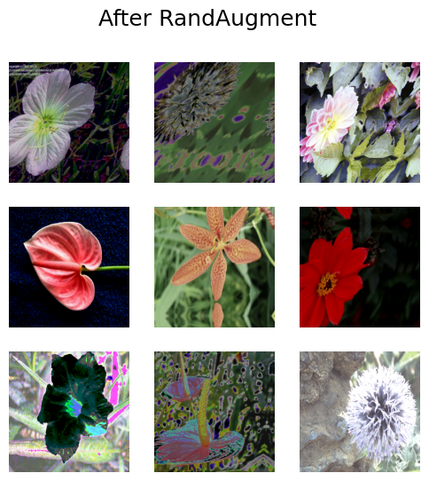
Try tweaking the magnitude settings to see a wider variety of results.
CutMix and MixUp: generate high-quality inter-class examples
CutMix and MixUp allow us to produce inter-class examples. CutMix randomly cuts out portions of one image and places them over another, and MixUp interpolates the pixel values between two images. Both of these prevent the model from overfitting the training distribution and improve the likelihood that the model can generalize to out of distribution examples. Additionally, CutMix prevents your model from over-relying on any particular feature to perform its classifications. You can read more about these techniques in their respective papers:
In this example, we will use CutMix and MixUp independently in a manually created preprocessing pipeline. In most state of the art pipelines images are randomly augmented by either CutMix, MixUp, or neither. The function below implements both.
cut_mix = keras_cv.layers.CutMix()
mix_up = keras_cv.layers.MixUp()


def cut_mix_and_mix_up(samples):
    samples = cut_mix(samples, training=True)
    samples = mix_up(samples, training=True)
    return samples


train_dataset = load_dataset().map(cut_mix_and_mix_up, num_parallel_calls=AUTOTUNE)

visualize_dataset(train_dataset, title="After CutMix and MixUp")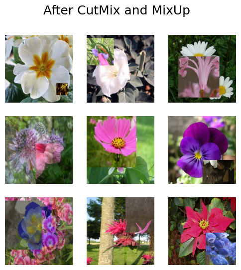
Great! Looks like we have successfully added CutMix and MixUp to our preprocessing pipeline.
Customizing your augmentation pipeline
Perhaps you want to exclude an augmentation from RandAugment, or perhaps you want to include the keras_cv.layers.GridMask as an option alongside the default RandAugment augmentations.
KerasCV allows you to construct production grade custom data augmentation pipelines using the keras_cv.layers.RandomAugmentationPipeline layer. This class operates similarly to RandAugment; selecting a random layer to apply to each image augmentations_per_image times. RandAugment can be thought of as a specific case of RandomAugmentationPipeline. In fact, our RandAugment implementation inherits from RandomAugmentationPipeline internally.
In this example, we will create a custom RandomAugmentationPipeline by removing RandomRotation layers from the standard RandAugment policy, and substitute a GridMask layer in its place.
As a first step, let’s use the helper method RandAugment.get_standard_policy() to create a base pipeline.
layers = keras_cv.layers.RandAugment.get_standard_policy(
    value_range=(0, 255), magnitude=0.75, magnitude_stddev=0.3
)
First, let’s filter out RandomRotation layers
layers = [
    layer for layer in layers if not isinstance(layer, keras_cv.layers.RandomRotation)
]
Next, let’s add keras_cv.layers.GridMask to our layers:
layers = layers + [keras_cv.layers.GridMask()]Finally, we can put together our pipeline
pipeline = keras_cv.layers.RandomAugmentationPipeline(
    layers=layers, augmentations_per_image=3
)


def apply_pipeline(inputs):
    inputs["images"] = pipeline(inputs["images"])
    return inputs
Let’s check out the results!
train_dataset = load_dataset().map(apply_pipeline, num_parallel_calls=AUTOTUNE)
visualize_dataset(train_dataset, title="After custom pipeline")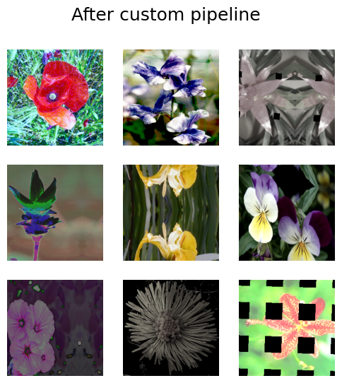
Awesome! As you can see, no images were randomly rotated. You can customize the pipeline however you like:
pipeline = keras_cv.layers.RandomAugmentationPipeline(
    layers=[keras_cv.layers.GridMask(), keras_cv.layers.Grayscale(output_channels=3)],
    augmentations_per_image=1,
)
This pipeline will either apply GrayScale or GridMask:
train_dataset = load_dataset().map(apply_pipeline, num_parallel_calls=AUTOTUNE)
visualize_dataset(train_dataset, title="After custom pipeline")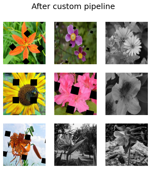
Looks great! You can use RandomAugmentationPipeline however you want.
Training a CNN
As a final exercise, let’s take some of these layers for a spin. In this section, we will use CutMix, MixUp, and RandAugment to train a state of the art ResNet50 image classifier on the Oxford flowers dataset.
def preprocess_for_model(inputs):
    images, labels = inputs["images"], inputs["labels"]
    images = tf.cast(images, tf.float32)
    return images, labels


train_dataset = (
    load_dataset()
    .map(apply_rand_augment, num_parallel_calls=AUTOTUNE)
    .map(cut_mix_and_mix_up, num_parallel_calls=AUTOTUNE)
)

visualize_dataset(train_dataset, "CutMix, MixUp and RandAugment")

train_dataset = train_dataset.map(preprocess_for_model, num_parallel_calls=AUTOTUNE)

test_dataset = load_dataset(split="test")
test_dataset = test_dataset.map(preprocess_for_model, num_parallel_calls=AUTOTUNE)

train_dataset = train_dataset.prefetch(AUTOTUNE)
test_dataset = test_dataset.prefetch(AUTOTUNE)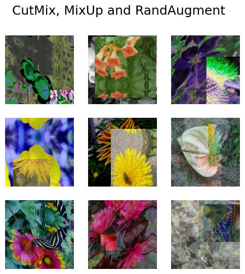
Next we should create a the model itself. Notice that we use label_smoothing=0.1 in the loss function. When using MixUp, label smoothing is highly recommended.
input_shape = IMAGE_SIZE + (3,)


def get_model():
    model = keras_cv.models.ImageClassifier.from_preset(
        "efficientnetv2_s", num_classes=num_classes
    )
    model.compile(
        loss=keras.losses.CategoricalCrossentropy(label_smoothing=0.1),
        optimizer=keras.optimizers.SGD(momentum=0.9),
        metrics=["accuracy"],
    )
    return model
Finally we train the model:
model = get_model()
model.fit(
    train_dataset,
    epochs=1,
    validation_data=test_dataset,
)
Result
 32/32 ━━━━━━━━━━━━━━━━━━━━ 103s 2s/step - accuracy: 0.0059 - loss: 4.6941 - val_accuracy: 0.0114 - val_loss: 10.4028

<keras.src.callbacks.history.History at 0x7fd0d00e07c0>
Conclusion & next steps
That’s all it takes to assemble state of the art image augmentation pipeliens with KerasCV!
As an additional exercise for readers, you can:
- Perform a hyper parameter search over the RandAugment parameters to improve the classifier accuracy
- Substitute the Oxford Flowers dataset with your own dataset
- Experiment with custom
RandomAugmentationPipelineobjects.
Currently, between Keras core and KerasCV there are 28 image augmentation layers! Each of these can be used independently, or in a pipeline. Check them out, and if you find an augmentation techniques you need is missing please file a GitHub issue on KerasCV.