Drug Molecule Generation with VAE
- Original Link : https://keras.io/examples/generative/molecule_generation/
- Last Checked at : 2024-11-23
Author: Victor Basu
Date created: 2022/03/10
Last modified: 2022/03/24
Description: Implementing a Convolutional Variational AutoEncoder (VAE) for Drug Discovery.
Introduction
In this example, we use a Variational Autoencoder to generate molecules for drug discovery. We use the research papers Automatic chemical design using a data-driven continuous representation of molecules and MolGAN: An implicit generative model for small molecular graphs as a reference.
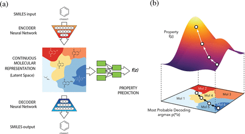
The model described in the paper Automatic chemical design using a data-driven continuous representation of molecules generates new molecules via efficient exploration of open-ended spaces of chemical compounds. The model consists of three components: Encoder, Decoder and Predictor. The Encoder converts the discrete representation of a molecule into a real-valued continuous vector, and the Decoder converts these continuous vectors back to discrete molecule representations. The Predictor estimates chemical properties from the latent continuous vector representation of the molecule. Continuous representations allow the use of gradient-based optimization to efficiently guide the search for optimized functional compounds.

Figure (a) - A diagram of the autoencoder used for molecule design, including the joint property prediction model. Starting from a discrete molecule representation, such as a SMILES string, the encoder network converts each molecule into a vector in the latent space, which is effectively a continuous molecule representation. Given a point in the latent space, the decoder network produces a corresponding SMILES string. A multilayer perceptron network estimates the value of target properties associated with each molecule.
Figure (b) - Gradient-based optimization in continuous latent space. After training a surrogate model f(z) to predict the properties of molecules based on their latent representation z, we can optimize f(z) with respect to z to find new latent representations expected to match specific desired properties. These new latent representations can then be decoded into SMILES strings, at which point their properties can be tested empirically.
For an explanation and implementation of MolGAN, please refer to the Keras Example WGAN-GP with R-GCN for the generation of small molecular graphs by Alexander Kensert. Many of the functions used in the present example are from the above Keras example.
Setup
RDKit is an open source toolkit for cheminformatics and machine learning. This toolkit come in handy if one is into drug discovery domain. In this example, RDKit is used to conveniently and efficiently transform SMILES to molecule objects, and then from those obtain sets of atoms and bonds.
Quoting from WGAN-GP with R-GCN for the generation of small molecular graphs:
“SMILES expresses the structure of a given molecule in the form of an ASCII string. The SMILES string is a compact encoding which, for smaller molecules, is relatively human-readable. Encoding molecules as a string both alleviates and facilitates database and/or web searching of a given molecule. RDKit uses algorithms to accurately transform a given SMILES to a molecule object, which can then be used to compute a great number of molecular properties/features.”
!pip -q install rdkit-pypi==2021.9.4import ast
import pandas as pd
import numpy as np
import tensorflow as tf
from tensorflow import keras
from tensorflow.keras import layers
import matplotlib.pyplot as plt
from rdkit import Chem, RDLogger
from rdkit.Chem import BondType
from rdkit.Chem.Draw import MolsToGridImage
RDLogger.DisableLog("rdApp.*")Result
[K |████████████████████████████████| 20.6 MB 1.2 MB/s
[?25hDataset
We use the ZINC – A Free Database of Commercially Available Compounds for Virtual Screening dataset. The dataset comes with molecule formula in SMILE representation along with their respective molecular properties such as logP (water–octanal partition coefficient), SAS (synthetic accessibility score) and QED (Qualitative Estimate of Drug-likeness).
csv_path = keras.utils.get_file(
    "/content/250k_rndm_zinc_drugs_clean_3.csv",
    "https://raw.githubusercontent.com/aspuru-guzik-group/chemical_vae/master/models/zinc_properties/250k_rndm_zinc_drugs_clean_3.csv",
)

df = pd.read_csv("/content/250k_rndm_zinc_drugs_clean_3.csv")
df["smiles"] = df["smiles"].apply(lambda s: s.replace("\n", ""))
df.head()
Result
Downloading data from https://raw.githubusercontent.com/aspuru-guzik-group/chemical_vae/master/models/zinc_properties/250k_rndm_zinc_drugs_clean_3.csv
22606589/22606589 [==============================] - 0s 0us/step| smiles | logP | qed | SAS | |
|---|---|---|---|---|
| 0 | CC(C)(C)c1ccc2occ(CC(=O)Nc3ccccc3F)c2c1 | 5.05060 | 0.702012 | 2.084095 |
| 1 | C[C@@H]1CC(Nc2cncc(-c3nncn3C)c2)C[C@@H](C)C1 | 3.11370 | 0.928975 | 3.432004 |
| 2 | N#Cc1ccc(-c2ccc(O[C@@H](C(=O)N3CCCC3)c3ccccc3)… | 4.96778 | 0.599682 | 2.470633 |
| 3 | CCOC(=O)[C@@H]1CCCN(C(=O)c2nc(-c3ccc(C)cc3)n3c… | 4.00022 | 0.690944 | 2.822753 |
| 4 | N#CC1=C(SCC(=O)Nc2cccc(Cl)c2)N=C([O-])[C@H](C#… | 3.60956 | 0.789027 | 4.035182 |
Hyperparameters
SMILE_CHARSET = '["C", "B", "F", "I", "H", "O", "N", "S", "P", "Cl", "Br"]'

bond_mapping = {"SINGLE": 0, "DOUBLE": 1, "TRIPLE": 2, "AROMATIC": 3}
bond_mapping.update(
    {0: BondType.SINGLE, 1: BondType.DOUBLE, 2: BondType.TRIPLE, 3: BondType.AROMATIC}
)
SMILE_CHARSET = ast.literal_eval(SMILE_CHARSET)

MAX_MOLSIZE = max(df["smiles"].str.len())
SMILE_to_index = dict((c, i) for i, c in enumerate(SMILE_CHARSET))
index_to_SMILE = dict((i, c) for i, c in enumerate(SMILE_CHARSET))
atom_mapping = dict(SMILE_to_index)
atom_mapping.update(index_to_SMILE)

BATCH_SIZE = 100
EPOCHS = 10

VAE_LR = 5e-4
NUM_ATOMS = 120  # Maximum number of atoms

ATOM_DIM = len(SMILE_CHARSET)  # Number of atom types
BOND_DIM = 4 + 1  # Number of bond types
LATENT_DIM = 435  # Size of the latent space


def smiles_to_graph(smiles):
    # Converts SMILES to molecule object
    molecule = Chem.MolFromSmiles(smiles)

    # Initialize adjacency and feature tensor
    adjacency = np.zeros((BOND_DIM, NUM_ATOMS, NUM_ATOMS), "float32")
    features = np.zeros((NUM_ATOMS, ATOM_DIM), "float32")

    # loop over each atom in molecule
    for atom in molecule.GetAtoms():
        i = atom.GetIdx()
        atom_type = atom_mapping[atom.GetSymbol()]
        features[i] = np.eye(ATOM_DIM)[atom_type]
        # loop over one-hop neighbors
        for neighbor in atom.GetNeighbors():
            j = neighbor.GetIdx()
            bond = molecule.GetBondBetweenAtoms(i, j)
            bond_type_idx = bond_mapping[bond.GetBondType().name]
            adjacency[bond_type_idx, [i, j], [j, i]] = 1

    # Where no bond, add 1 to last channel (indicating "non-bond")
    # Notice: channels-first
    adjacency[-1, np.sum(adjacency, axis=0) == 0] = 1

    # Where no atom, add 1 to last column (indicating "non-atom")
    features[np.where(np.sum(features, axis=1) == 0)[0], -1] = 1

    return adjacency, features


def graph_to_molecule(graph):
    # Unpack graph
    adjacency, features = graph

    # RWMol is a molecule object intended to be edited
    molecule = Chem.RWMol()

    # Remove "no atoms" & atoms with no bonds
    keep_idx = np.where(
        (np.argmax(features, axis=1) != ATOM_DIM - 1)
        & (np.sum(adjacency[:-1], axis=(0, 1)) != 0)
    )[0]
    features = features[keep_idx]
    adjacency = adjacency[:, keep_idx, :][:, :, keep_idx]

    # Add atoms to molecule
    for atom_type_idx in np.argmax(features, axis=1):
        atom = Chem.Atom(atom_mapping[atom_type_idx])
        _ = molecule.AddAtom(atom)

    # Add bonds between atoms in molecule; based on the upper triangles
    # of the [symmetric] adjacency tensor
    (bonds_ij, atoms_i, atoms_j) = np.where(np.triu(adjacency) == 1)
    for (bond_ij, atom_i, atom_j) in zip(bonds_ij, atoms_i, atoms_j):
        if atom_i == atom_j or bond_ij == BOND_DIM - 1:
            continue
        bond_type = bond_mapping[bond_ij]
        molecule.AddBond(int(atom_i), int(atom_j), bond_type)

    # Sanitize the molecule; for more information on sanitization, see
    # https://www.rdkit.org/docs/RDKit_Book.html#molecular-sanitization
    flag = Chem.SanitizeMol(molecule, catchErrors=True)
    # Let's be strict. If sanitization fails, return None
    if flag != Chem.SanitizeFlags.SANITIZE_NONE:
        return None

    return molecule
Generate training set
train_df = df.sample(frac=0.75, random_state=42)  # random state is a seed value
train_df.reset_index(drop=True, inplace=True)

adjacency_tensor, feature_tensor, qed_tensor = [], [], []
for idx in range(8000):
    adjacency, features = smiles_to_graph(train_df.loc[idx]["smiles"])
    qed = train_df.loc[idx]["qed"]
    adjacency_tensor.append(adjacency)
    feature_tensor.append(features)
    qed_tensor.append(qed)

adjacency_tensor = np.array(adjacency_tensor)
feature_tensor = np.array(feature_tensor)
qed_tensor = np.array(qed_tensor)


class RelationalGraphConvLayer(keras.layers.Layer):
    def __init__(
        self,
        units=128,
        activation="relu",
        use_bias=False,
        kernel_initializer="glorot_uniform",
        bias_initializer="zeros",
        kernel_regularizer=None,
        bias_regularizer=None,
        **kwargs
    ):
        super().__init__(**kwargs)

        self.units = units
        self.activation = keras.activations.get(activation)
        self.use_bias = use_bias
        self.kernel_initializer = keras.initializers.get(kernel_initializer)
        self.bias_initializer = keras.initializers.get(bias_initializer)
        self.kernel_regularizer = keras.regularizers.get(kernel_regularizer)
        self.bias_regularizer = keras.regularizers.get(bias_regularizer)

    def build(self, input_shape):
        bond_dim = input_shape[0][1]
        atom_dim = input_shape[1][2]

        self.kernel = self.add_weight(
            shape=(bond_dim, atom_dim, self.units),
            initializer=self.kernel_initializer,
            regularizer=self.kernel_regularizer,
            trainable=True,
            name="W",
            dtype=tf.float32,
        )

        if self.use_bias:
            self.bias = self.add_weight(
                shape=(bond_dim, 1, self.units),
                initializer=self.bias_initializer,
                regularizer=self.bias_regularizer,
                trainable=True,
                name="b",
                dtype=tf.float32,
            )

        self.built = True

    def call(self, inputs, training=False):
        adjacency, features = inputs
        # Aggregate information from neighbors
        x = tf.matmul(adjacency, features[:, None, :, :])
        # Apply linear transformation
        x = tf.matmul(x, self.kernel)
        if self.use_bias:
            x += self.bias
        # Reduce bond types dim
        x_reduced = tf.reduce_sum(x, axis=1)
        # Apply non-linear transformation
        return self.activation(x_reduced)
Build the Encoder and Decoder
The Encoder takes as input a molecule’s graph adjacency matrix and feature matrix. These features are processed via a Graph Convolution layer, then are flattened and processed by several Dense layers to derive z_mean and log_var, the latent-space representation of the molecule.
Graph Convolution layer: The relational graph convolution layer implements non-linearly transformed neighbourhood aggregations. We can define these layers as follows:
$$ H^{l+1} = σ(D^{-1} @ A @ H^{l+1} @ W^{l}) $$
Where $\sigma$ denotes the non-linear transformation (commonly a ReLU activation), $A$ the adjacency tensor, $H^{l}$ the feature tensor at the l-th layer, $D^{-1}$ the inverse diagonal degree tensor of $A^$, and $W^{l}$ the trainable weight tensor at the l-th layer. Specifically, for each bond type (relation), the degree tensor expresses, in the diagonal, the number of bonds attached to each atom.
Source: WGAN-GP with R-GCN for the generation of small molecular graphs
The Decoder takes as input the latent-space representation and predicts the graph adjacency matrix and feature matrix of the corresponding molecules.
def get_encoder(
    gconv_units, latent_dim, adjacency_shape, feature_shape, dense_units, dropout_rate
):
    adjacency = keras.layers.Input(shape=adjacency_shape)
    features = keras.layers.Input(shape=feature_shape)

    # Propagate through one or more graph convolutional layers
    features_transformed = features
    for units in gconv_units:
        features_transformed = RelationalGraphConvLayer(units)(
            [adjacency, features_transformed]
        )
    # Reduce 2-D representation of molecule to 1-D
    x = keras.layers.GlobalAveragePooling1D()(features_transformed)

    # Propagate through one or more densely connected layers
    for units in dense_units:
        x = layers.Dense(units, activation="relu")(x)
        x = layers.Dropout(dropout_rate)(x)

    z_mean = layers.Dense(latent_dim, dtype="float32", name="z_mean")(x)
    log_var = layers.Dense(latent_dim, dtype="float32", name="log_var")(x)

    encoder = keras.Model([adjacency, features], [z_mean, log_var], name="encoder")

    return encoder


def get_decoder(dense_units, dropout_rate, latent_dim, adjacency_shape, feature_shape):
    latent_inputs = keras.Input(shape=(latent_dim,))

    x = latent_inputs
    for units in dense_units:
        x = keras.layers.Dense(units, activation="tanh")(x)
        x = keras.layers.Dropout(dropout_rate)(x)

    # Map outputs of previous layer (x) to [continuous] adjacency tensors (x_adjacency)
    x_adjacency = keras.layers.Dense(tf.math.reduce_prod(adjacency_shape))(x)
    x_adjacency = keras.layers.Reshape(adjacency_shape)(x_adjacency)
    # Symmetrify tensors in the last two dimensions
    x_adjacency = (x_adjacency + tf.transpose(x_adjacency, (0, 1, 3, 2))) / 2
    x_adjacency = keras.layers.Softmax(axis=1)(x_adjacency)

    # Map outputs of previous layer (x) to [continuous] feature tensors (x_features)
    x_features = keras.layers.Dense(tf.math.reduce_prod(feature_shape))(x)
    x_features = keras.layers.Reshape(feature_shape)(x_features)
    x_features = keras.layers.Softmax(axis=2)(x_features)

    decoder = keras.Model(
        latent_inputs, outputs=[x_adjacency, x_features], name="decoder"
    )

    return decoder
Build the Sampling layer
class Sampling(layers.Layer):
    def call(self, inputs):
        z_mean, z_log_var = inputs
        batch = tf.shape(z_log_var)[0]
        dim = tf.shape(z_log_var)[1]
        epsilon = tf.keras.backend.random_normal(shape=(batch, dim))
        return z_mean + tf.exp(0.5 * z_log_var) * epsilon
Build the VAE
This model is trained to optimize four losses:
- Categorical crossentropy
- KL divergence loss
- Property prediction loss
- Graph loss (gradient penalty)
The categorical crossentropy loss function measures the model’s reconstruction accuracy. The Property prediction loss estimates the mean squared error between predicted and actual properties after running the latent representation through a property prediction model. The property prediction of the model is optimized via binary crossentropy. The gradient penalty is further guided by the model’s property (QED) prediction.
A gradient penalty is an alternative soft constraint on the 1-Lipschitz continuity as an improvement upon the gradient clipping scheme from the original neural network (“1-Lipschitz continuity” means that the norm of the gradient is at most 1 at every single point of the function). It adds a regularization term to the loss function.
class MoleculeGenerator(keras.Model):
    def __init__(self, encoder, decoder, max_len, **kwargs):
        super().__init__(**kwargs)
        self.encoder = encoder
        self.decoder = decoder
        self.property_prediction_layer = layers.Dense(1)
        self.max_len = max_len

        self.train_total_loss_tracker = keras.metrics.Mean(name="train_total_loss")
        self.val_total_loss_tracker = keras.metrics.Mean(name="val_total_loss")

    def train_step(self, data):
        adjacency_tensor, feature_tensor, qed_tensor = data[0]
        graph_real = [adjacency_tensor, feature_tensor]
        self.batch_size = tf.shape(qed_tensor)[0]
        with tf.GradientTape() as tape:
            z_mean, z_log_var, qed_pred, gen_adjacency, gen_features = self(
                graph_real, training=True
            )
            graph_generated = [gen_adjacency, gen_features]
            total_loss = self._compute_loss(
                z_log_var, z_mean, qed_tensor, qed_pred, graph_real, graph_generated
            )

        grads = tape.gradient(total_loss, self.trainable_weights)
        self.optimizer.apply_gradients(zip(grads, self.trainable_weights))

        self.train_total_loss_tracker.update_state(total_loss)
        return {"loss": self.train_total_loss_tracker.result()}

    def _compute_loss(
        self, z_log_var, z_mean, qed_true, qed_pred, graph_real, graph_generated
    ):

        adjacency_real, features_real = graph_real
        adjacency_gen, features_gen = graph_generated

        adjacency_loss = tf.reduce_mean(
            tf.reduce_sum(
                keras.losses.categorical_crossentropy(adjacency_real, adjacency_gen),
                axis=(1, 2),
            )
        )
        features_loss = tf.reduce_mean(
            tf.reduce_sum(
                keras.losses.categorical_crossentropy(features_real, features_gen),
                axis=(1),
            )
        )
        kl_loss = -0.5 * tf.reduce_sum(
            1 + z_log_var - tf.square(z_mean) - tf.exp(z_log_var), 1
        )
        kl_loss = tf.reduce_mean(kl_loss)

        property_loss = tf.reduce_mean(
            keras.losses.binary_crossentropy(qed_true, qed_pred)
        )

        graph_loss = self._gradient_penalty(graph_real, graph_generated)

        return kl_loss + property_loss + graph_loss + adjacency_loss + features_loss

    def _gradient_penalty(self, graph_real, graph_generated):
        # Unpack graphs
        adjacency_real, features_real = graph_real
        adjacency_generated, features_generated = graph_generated

        # Generate interpolated graphs (adjacency_interp and features_interp)
        alpha = tf.random.uniform([self.batch_size])
        alpha = tf.reshape(alpha, (self.batch_size, 1, 1, 1))
        adjacency_interp = (adjacency_real * alpha) + (1 - alpha) * adjacency_generated
        alpha = tf.reshape(alpha, (self.batch_size, 1, 1))
        features_interp = (features_real * alpha) + (1 - alpha) * features_generated

        # Compute the logits of interpolated graphs
        with tf.GradientTape() as tape:
            tape.watch(adjacency_interp)
            tape.watch(features_interp)
            _, _, logits, _, _ = self(
                [adjacency_interp, features_interp], training=True
            )

        # Compute the gradients with respect to the interpolated graphs
        grads = tape.gradient(logits, [adjacency_interp, features_interp])
        # Compute the gradient penalty
        grads_adjacency_penalty = (1 - tf.norm(grads[0], axis=1)) ** 2
        grads_features_penalty = (1 - tf.norm(grads[1], axis=2)) ** 2
        return tf.reduce_mean(
            tf.reduce_mean(grads_adjacency_penalty, axis=(-2, -1))
            + tf.reduce_mean(grads_features_penalty, axis=(-1))
        )

    def inference(self, batch_size):
        z = tf.random.normal((batch_size, LATENT_DIM))
        reconstruction_adjacency, reconstruction_features = model.decoder.predict(z)
        # obtain one-hot encoded adjacency tensor
        adjacency = tf.argmax(reconstruction_adjacency, axis=1)
        adjacency = tf.one_hot(adjacency, depth=BOND_DIM, axis=1)
        # Remove potential self-loops from adjacency
        adjacency = tf.linalg.set_diag(adjacency, tf.zeros(tf.shape(adjacency)[:-1]))
        # obtain one-hot encoded feature tensor
        features = tf.argmax(reconstruction_features, axis=2)
        features = tf.one_hot(features, depth=ATOM_DIM, axis=2)
        return [
            graph_to_molecule([adjacency[i].numpy(), features[i].numpy()])
            for i in range(batch_size)
        ]

    def call(self, inputs):
        z_mean, log_var = self.encoder(inputs)
        z = Sampling()([z_mean, log_var])

        gen_adjacency, gen_features = self.decoder(z)

        property_pred = self.property_prediction_layer(z_mean)

        return z_mean, log_var, property_pred, gen_adjacency, gen_features
Train the model
vae_optimizer = tf.keras.optimizers.Adam(learning_rate=VAE_LR)

encoder = get_encoder(
    gconv_units=[9],
    adjacency_shape=(BOND_DIM, NUM_ATOMS, NUM_ATOMS),
    feature_shape=(NUM_ATOMS, ATOM_DIM),
    latent_dim=LATENT_DIM,
    dense_units=[512],
    dropout_rate=0.0,
)
decoder = get_decoder(
    dense_units=[128, 256, 512],
    dropout_rate=0.2,
    latent_dim=LATENT_DIM,
    adjacency_shape=(BOND_DIM, NUM_ATOMS, NUM_ATOMS),
    feature_shape=(NUM_ATOMS, ATOM_DIM),
)

model = MoleculeGenerator(encoder, decoder, MAX_MOLSIZE)

model.compile(vae_optimizer)
history = model.fit([adjacency_tensor, feature_tensor, qed_tensor], epochs=EPOCHS)
Result
Epoch 1/10
250/250 [==============================] - 24s 84ms/step - loss: 68958.3946
Epoch 2/10
250/250 [==============================] - 20s 79ms/step - loss: 68819.8421
Epoch 3/10
250/250 [==============================] - 20s 79ms/step - loss: 68830.6720
Epoch 4/10
250/250 [==============================] - 20s 79ms/step - loss: 68816.1486
Epoch 5/10
250/250 [==============================] - 20s 79ms/step - loss: 68825.9977
Epoch 6/10
250/250 [==============================] - 19s 78ms/step - loss: 68818.0771
Epoch 7/10
250/250 [==============================] - 19s 77ms/step - loss: 68815.8525
Epoch 8/10
250/250 [==============================] - 20s 78ms/step - loss: 68820.5459
Epoch 9/10
250/250 [==============================] - 21s 83ms/step - loss: 68806.9465
Epoch 10/10
250/250 [==============================] - 21s 84ms/step - loss: 68805.9879
Inference
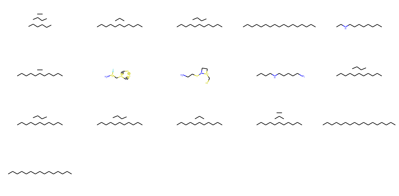
We use our model to generate new valid molecules from different points of the latent space.
Generate unique Molecules with the model
molecules = model.inference(1000)

MolsToGridImage(
    [m for m in molecules if m is not None][:1000], molsPerRow=5, subImgSize=(260, 160)
)
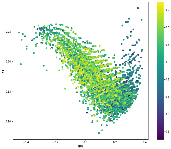
Display latent space clusters with respect to molecular properties (QAE)
def plot_latent(vae, data, labels):
    # display a 2D plot of the property in the latent space
    z_mean, _ = vae.encoder.predict(data)
    plt.figure(figsize=(12, 10))
    plt.scatter(z_mean[:, 0], z_mean[:, 1], c=labels)
    plt.colorbar()
    plt.xlabel("z[0]")
    plt.ylabel("z[1]")
    plt.show()


plot_latent(model, [adjacency_tensor[:8000], feature_tensor[:8000]], qed_tensor[:8000])
Conclusion
In this example, we combined model architectures from two papers, “Automatic chemical design using a data-driven continuous representation of molecules” from 2016 and the “MolGAN” paper from 2018. The former paper treats SMILES inputs as strings and seeks to generate molecule strings in SMILES format, while the later paper considers SMILES inputs as graphs (a combination of adjacency matrices and feature matrices) and seeks to generate molecules as graphs.
This hybrid approach enables a new type of directed gradient-based search through chemical space.
Example available on HuggingFace
| Trained Model | Demo |
|---|---|
 |  |