GauGAN for conditional image generation
- Original Link : https://keras.io/examples/generative/gaugan/
- Last Checked at : 2024-11-23
Author: Soumik Rakshit, Sayak Paul
Date created: 2021/12/26
Last modified: 2022/01/03
Description: Implementing a GauGAN for conditional image generation.
Introduction
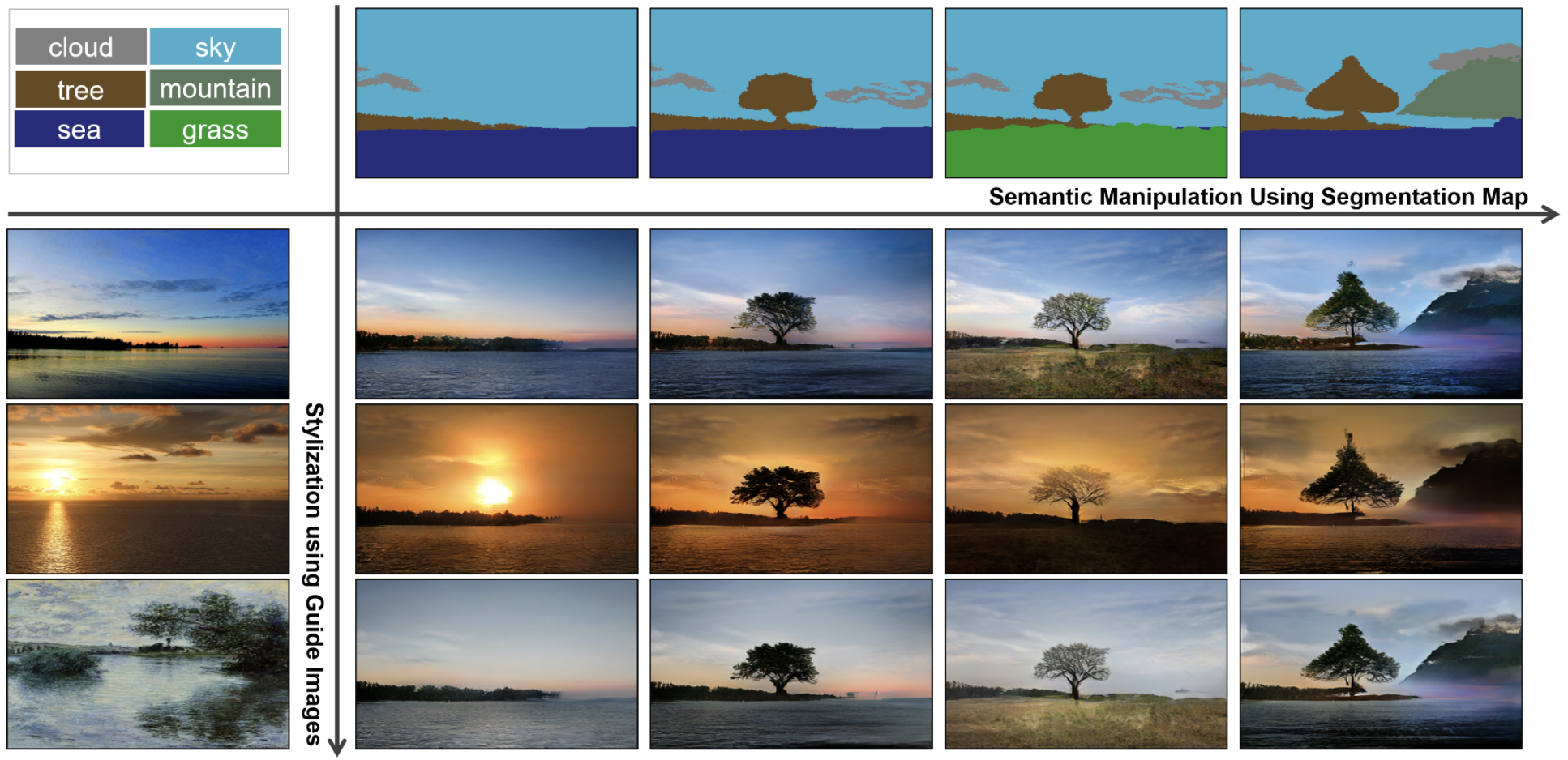
In this example, we present an implementation of the GauGAN architecture proposed in Semantic Image Synthesis with Spatially-Adaptive Normalization. Briefly, GauGAN uses a Generative Adversarial Network (GAN) to generate realistic images that are conditioned on cue images and segmentation maps, as shown below (image source):
The main components of a GauGAN are:
- SPADE (aka spatially-adaptive normalization) : The authors of GauGAN argue that the more conventional normalization layers (such as Batch Normalization) destroy the semantic information obtained from segmentation maps that are provided as inputs. To address this problem, the authors introduce SPADE, a normalization layer particularly suitable for learning affine parameters (scale and bias) that are spatially adaptive. This is done by learning different sets of scaling and bias parameters for each semantic label.
- Variational encoder: Inspired by Variational Autoencoders, GauGAN uses a variational formulation wherein an encoder learns the mean and variance of a normal (Gaussian) distribution from the cue images. This is where GauGAN gets its name from. The generator of GauGAN takes as inputs the latents sampled from the Gaussian distribution as well as the one-hot encoded semantic segmentation label maps. The cue images act as style images that guide the generator to stylistic generation. This variational formulation helps GauGAN achieve image diversity as well as fidelity.
- Multi-scale patch discriminator : Inspired by the PatchGAN model, GauGAN uses a discriminator that assesses a given image on a patch basis and produces an averaged score.
As we proceed with the example, we will discuss each of the different components in further detail.
For a thorough review of GauGAN, please refer to this article. We also encourage you to check out the official GauGAN website, which has many creative applications of GauGAN. This example assumes that the reader is already familiar with the fundamental concepts of GANs. If you need a refresher, the following resources might be useful:
- Chapter on GANs from the Deep Learning with Python book by François Chollet.
- GAN implementations on keras.io:
Data collection
We will be using the Facades dataset for training our GauGAN model. Let’s first download it.
!wget https://drive.google.com/uc?id=1q4FEjQg1YSb4mPx2VdxL7LXKYu3voTMj -O facades_data.zip
!unzip -q facades_data.zip
Result
--2024-01-11 22:46:32--  https://drive.google.com/uc?id=1q4FEjQg1YSb4mPx2VdxL7LXKYu3voTMj
Resolving drive.google.com (drive.google.com)... 64.233.181.138, 64.233.181.102, 64.233.181.100, ...
Connecting to drive.google.com (drive.google.com)|64.233.181.138|:443... connected.
HTTP request sent, awaiting response... 303 See Other
Location: https://drive.usercontent.google.com/download?id=1q4FEjQg1YSb4mPx2VdxL7LXKYu3voTMj [following]
--2024-01-11 22:46:32--  https://drive.usercontent.google.com/download?id=1q4FEjQg1YSb4mPx2VdxL7LXKYu3voTMj
Resolving drive.usercontent.google.com (drive.usercontent.google.com)... 108.177.112.132, 2607:f8b0:4001:c12::84
Connecting to drive.usercontent.google.com (drive.usercontent.google.com)|108.177.112.132|:443... connected.
HTTP request sent, awaiting response... 200 OK
Length: 26036052 (25M) [application/octet-stream]
Saving to: ‘facades_data.zip’
facades_data.zip    100%[===================>]  24.83M  94.3MB/s    in 0.3s
2024-01-11 22:46:42 (94.3 MB/s) - ‘facades_data.zip’ saved [26036052/26036052]
Imports
import os

os.environ["KERAS_BACKEND"] = "tensorflow"


import numpy as np
import matplotlib.pyplot as plt

import tensorflow as tf
import keras
from keras import ops
from keras import layers

from glob import glob
Data splitting
PATH = "./facades_data/"
SPLIT = 0.2

files = glob(PATH + "*.jpg")
np.random.shuffle(files)

split_index = int(len(files) * (1 - SPLIT))
train_files = files[:split_index]
val_files = files[split_index:]

print(f"Total samples: {len(files)}.")
print(f"Total training samples: {len(train_files)}.")
print(f"Total validation samples: {len(val_files)}.")
Result
Total samples: 378.
Total training samples: 302.
Total validation samples: 76.
Data loader
BATCH_SIZE = 4
IMG_HEIGHT = IMG_WIDTH = 256
NUM_CLASSES = 12
AUTOTUNE = tf.data.AUTOTUNE


def load(image_files, batch_size, is_train=True):
    def _random_crop(
        segmentation_map,
        image,
        labels,
        crop_size=(IMG_HEIGHT, IMG_WIDTH),
    ):
        crop_size = tf.convert_to_tensor(crop_size)
        image_shape = tf.shape(image)[:2]
        margins = image_shape - crop_size
        y1 = tf.random.uniform(shape=(), maxval=margins[0], dtype=tf.int32)
        x1 = tf.random.uniform(shape=(), maxval=margins[1], dtype=tf.int32)
        y2 = y1 + crop_size[0]
        x2 = x1 + crop_size[1]

        cropped_images = []
        images = [segmentation_map, image, labels]
        for img in images:
            cropped_images.append(img[y1:y2, x1:x2])
        return cropped_images

    def _load_data_tf(image_file, segmentation_map_file, label_file):
        image = tf.image.decode_png(tf.io.read_file(image_file), channels=3)
        segmentation_map = tf.image.decode_png(
            tf.io.read_file(segmentation_map_file), channels=3
        )
        labels = tf.image.decode_bmp(tf.io.read_file(label_file), channels=0)
        labels = tf.squeeze(labels)

        image = tf.cast(image, tf.float32) / 127.5 - 1
        segmentation_map = tf.cast(segmentation_map, tf.float32) / 127.5 - 1
        return segmentation_map, image, labels

    def _one_hot(segmentation_maps, real_images, labels):
        labels = tf.one_hot(labels, NUM_CLASSES)
        labels.set_shape((None, None, NUM_CLASSES))
        return segmentation_maps, real_images, labels

    segmentation_map_files = [
        image_file.replace("images", "segmentation_map").replace("jpg", "png")
        for image_file in image_files
    ]
    label_files = [
        image_file.replace("images", "segmentation_labels").replace("jpg", "bmp")
        for image_file in image_files
    ]
    dataset = tf.data.Dataset.from_tensor_slices(
        (image_files, segmentation_map_files, label_files)
    )

    dataset = dataset.shuffle(batch_size * 10) if is_train else dataset
    dataset = dataset.map(_load_data_tf, num_parallel_calls=AUTOTUNE)
    dataset = dataset.map(_random_crop, num_parallel_calls=AUTOTUNE)
    dataset = dataset.map(_one_hot, num_parallel_calls=AUTOTUNE)
    dataset = dataset.batch(batch_size, drop_remainder=True)
    return dataset


train_dataset = load(train_files, batch_size=BATCH_SIZE, is_train=True)
val_dataset = load(val_files, batch_size=BATCH_SIZE, is_train=False)
Now, let’s visualize a few samples from the training set.
sample_train_batch = next(iter(train_dataset))
print(f"Segmentation map batch shape: {sample_train_batch[0].shape}.")
print(f"Image batch shape: {sample_train_batch[1].shape}.")
print(f"One-hot encoded label map shape: {sample_train_batch[2].shape}.")

# Plot a view samples from the training set.
for segmentation_map, real_image in zip(sample_train_batch[0], sample_train_batch[1]):
    fig = plt.figure(figsize=(10, 10))
    fig.add_subplot(1, 2, 1).set_title("Segmentation Map")
    plt.imshow((segmentation_map + 1) / 2)
    fig.add_subplot(1, 2, 2).set_title("Real Image")
    plt.imshow((real_image + 1) / 2)
    plt.show()
Result
Segmentation map batch shape: (4, 256, 256, 3).
Image batch shape: (4, 256, 256, 3).
One-hot encoded label map shape: (4, 256, 256, 12).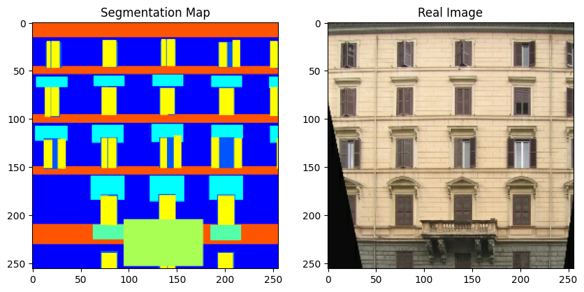
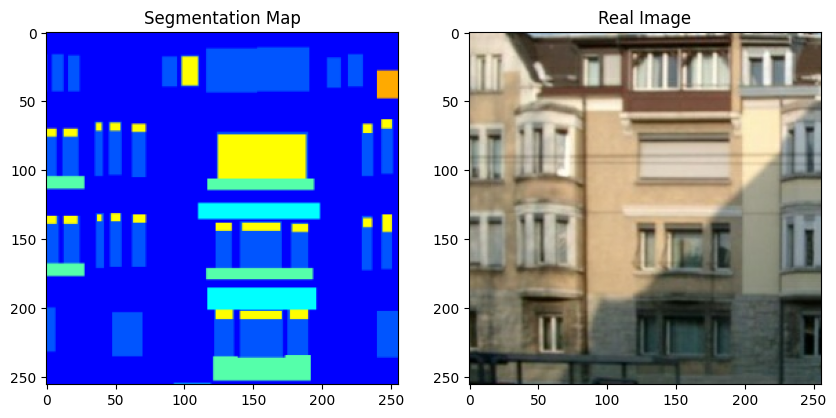
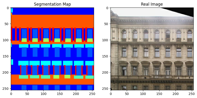
Note that in the rest of this example, we use a couple of figures from the original GauGAN paper for convenience.
Custom layers
In the following section, we implement the following layers:
- SPADE
- Residual block including SPADE
- Gaussian sampler
Some more notes on SPADE
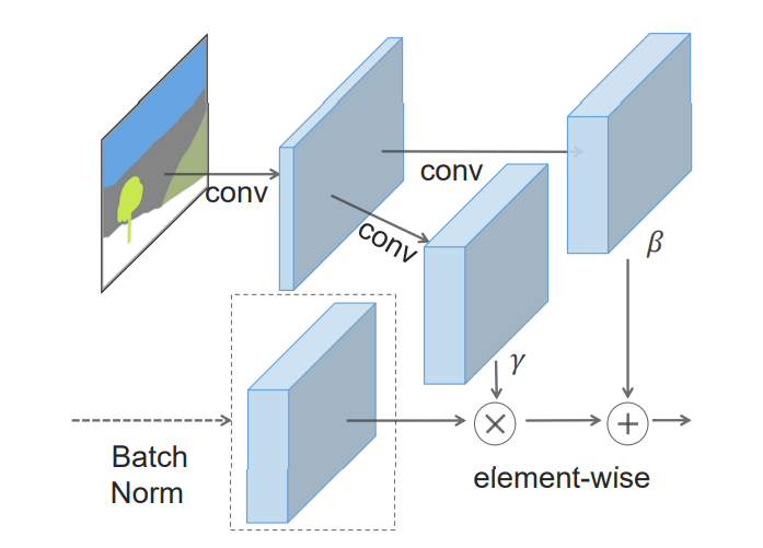
SPatially-Adaptive (DE) normalization or SPADE is a simple but effective layer for synthesizing photorealistic images given an input semantic layout. Previous methods for conditional image generation from semantic input such as Pix2Pix (Isola et al.) or Pix2PixHD (Wang et al.) directly feed the semantic layout as input to the deep network, which is then processed through stacks of convolution, normalization, and nonlinearity layers. This is often suboptimal as the normalization layers have a tendency to wash away semantic information.
In SPADE, the segmentation mask is first projected onto an embedding space, and then convolved to produce the modulation parameters γ and β. Unlike prior conditional normalization methods, γ and β are not vectors, but tensors with spatial dimensions. The produced γ and β are multiplied and added to the normalized activation element-wise. As the modulation parameters are adaptive to the input segmentation mask, SPADE is better suited for semantic image synthesis.
class SPADE(layers.Layer):
    def __init__(self, filters, epsilon=1e-5, **kwargs):
        super().__init__(**kwargs)
        self.epsilon = epsilon
        self.conv = layers.Conv2D(128, 3, padding="same", activation="relu")
        self.conv_gamma = layers.Conv2D(filters, 3, padding="same")
        self.conv_beta = layers.Conv2D(filters, 3, padding="same")

    def build(self, input_shape):
        self.resize_shape = input_shape[1:3]

    def call(self, input_tensor, raw_mask):
        mask = ops.image.resize(raw_mask, self.resize_shape, interpolation="nearest")
        x = self.conv(mask)
        gamma = self.conv_gamma(x)
        beta = self.conv_beta(x)
        mean, var = ops.moments(input_tensor, axes=(0, 1, 2), keepdims=True)
        std = ops.sqrt(var + self.epsilon)
        normalized = (input_tensor - mean) / std
        output = gamma * normalized + beta
        return output


class ResBlock(layers.Layer):
    def __init__(self, filters, **kwargs):
        super().__init__(**kwargs)
        self.filters = filters

    def build(self, input_shape):
        input_filter = input_shape[-1]
        self.spade_1 = SPADE(input_filter)
        self.spade_2 = SPADE(self.filters)
        self.conv_1 = layers.Conv2D(self.filters, 3, padding="same")
        self.conv_2 = layers.Conv2D(self.filters, 3, padding="same")
        self.learned_skip = False

        if self.filters != input_filter:
            self.learned_skip = True
            self.spade_3 = SPADE(input_filter)
            self.conv_3 = layers.Conv2D(self.filters, 3, padding="same")

    def call(self, input_tensor, mask):
        x = self.spade_1(input_tensor, mask)
        x = self.conv_1(keras.activations.leaky_relu(x, 0.2))
        x = self.spade_2(x, mask)
        x = self.conv_2(keras.activations.leaky_relu(x, 0.2))
        skip = (
            self.conv_3(
                keras.activations.leaky_relu(self.spade_3(input_tensor, mask), 0.2)
            )
            if self.learned_skip
            else input_tensor
        )
        output = skip + x
        return output


class GaussianSampler(layers.Layer):
    def __init__(self, batch_size, latent_dim, **kwargs):
        super().__init__(**kwargs)
        self.batch_size = batch_size
        self.latent_dim = latent_dim
        self.seed_generator = keras.random.SeedGenerator(1337)

    def call(self, inputs):
        means, variance = inputs
        epsilon = keras.random.normal(
            shape=(self.batch_size, self.latent_dim),
            mean=0.0,
            stddev=1.0,
            seed=self.seed_generator,
        )
        samples = means + ops.exp(0.5 * variance) * epsilon
        return samples
Next, we implement the downsampling block for the encoder.
def downsample(
    channels,
    kernels,
    strides=2,
    apply_norm=True,
    apply_activation=True,
    apply_dropout=False,
):
    block = keras.Sequential()
    block.add(
        layers.Conv2D(
            channels,
            kernels,
            strides=strides,
            padding="same",
            use_bias=False,
            kernel_initializer=keras.initializers.GlorotNormal(),
        )
    )
    if apply_norm:
        block.add(layers.GroupNormalization(groups=-1))
    if apply_activation:
        block.add(layers.LeakyReLU(0.2))
    if apply_dropout:
        block.add(layers.Dropout(0.5))
    return block
The GauGAN encoder consists of a few downsampling blocks. It outputs the mean and variance of a distribution.
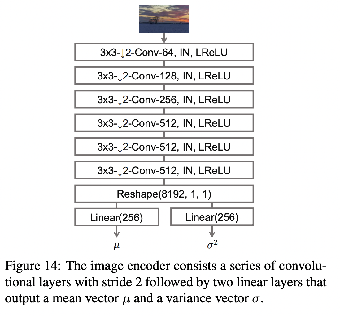
def build_encoder(image_shape, encoder_downsample_factor=64, latent_dim=256):
    input_image = keras.Input(shape=image_shape)
    x = downsample(encoder_downsample_factor, 3, apply_norm=False)(input_image)
    x = downsample(2 * encoder_downsample_factor, 3)(x)
    x = downsample(4 * encoder_downsample_factor, 3)(x)
    x = downsample(8 * encoder_downsample_factor, 3)(x)
    x = downsample(8 * encoder_downsample_factor, 3)(x)
    x = layers.Flatten()(x)
    mean = layers.Dense(latent_dim, name="mean")(x)
    variance = layers.Dense(latent_dim, name="variance")(x)
    return keras.Model(input_image, [mean, variance], name="encoder")
Next, we implement the generator, which consists of the modified residual blocks and upsampling blocks. It takes latent vectors and one-hot encoded segmentation labels, and produces new images.
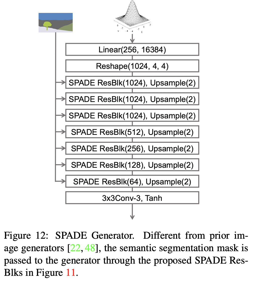
With SPADE, there is no need to feed the segmentation map to the first layer of the generator, since the latent inputs have enough structural information about the style we want the generator to emulate. We also discard the encoder part of the generator, which is commonly used in prior architectures. This results in a more lightweight generator network, which can also take a random vector as input, enabling a simple and natural path to multi-modal synthesis.
def build_generator(mask_shape, latent_dim=256):
    latent = keras.Input(shape=(latent_dim,))
    mask = keras.Input(shape=mask_shape)
    x = layers.Dense(16384)(latent)
    x = layers.Reshape((4, 4, 1024))(x)
    x = ResBlock(filters=1024)(x, mask)
    x = layers.UpSampling2D((2, 2))(x)
    x = ResBlock(filters=1024)(x, mask)
    x = layers.UpSampling2D((2, 2))(x)
    x = ResBlock(filters=1024)(x, mask)
    x = layers.UpSampling2D((2, 2))(x)
    x = ResBlock(filters=512)(x, mask)
    x = layers.UpSampling2D((2, 2))(x)
    x = ResBlock(filters=256)(x, mask)
    x = layers.UpSampling2D((2, 2))(x)
    x = ResBlock(filters=128)(x, mask)
    x = layers.UpSampling2D((2, 2))(x)
    x = keras.activations.leaky_relu(x, 0.2)
    output_image = keras.activations.tanh(layers.Conv2D(3, 4, padding="same")(x))
    return keras.Model([latent, mask], output_image, name="generator")
The discriminator takes a segmentation map and an image and concatenates them. It then predicts if patches of the concatenated image are real or fake.
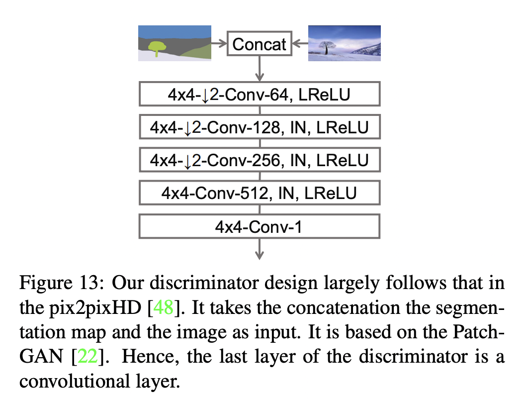
def build_discriminator(image_shape, downsample_factor=64):
    input_image_A = keras.Input(shape=image_shape, name="discriminator_image_A")
    input_image_B = keras.Input(shape=image_shape, name="discriminator_image_B")
    x = layers.Concatenate()([input_image_A, input_image_B])
    x1 = downsample(downsample_factor, 4, apply_norm=False)(x)
    x2 = downsample(2 * downsample_factor, 4)(x1)
    x3 = downsample(4 * downsample_factor, 4)(x2)
    x4 = downsample(8 * downsample_factor, 4, strides=1)(x3)
    x5 = layers.Conv2D(1, 4)(x4)
    outputs = [x1, x2, x3, x4, x5]
    return keras.Model([input_image_A, input_image_B], outputs)
Loss functions
GauGAN uses the following loss functions:
Generator:
- Expectation over the discriminator predictions.
- KL divergence for learning the mean and variance predicted by the encoder.
- Minimization between the discriminator predictions on original and generated images to align the feature space of the generator.
- Perceptual loss for encouraging the generated images to have perceptual quality.
Discriminator:
def generator_loss(y):
    return -ops.mean(y)


def kl_divergence_loss(mean, variance):
    return -0.5 * ops.sum(1 + variance - ops.square(mean) - ops.exp(variance))


class FeatureMatchingLoss(keras.losses.Loss):
    def __init__(self, **kwargs):
        super().__init__(**kwargs)
        self.mae = keras.losses.MeanAbsoluteError()

    def call(self, y_true, y_pred):
        loss = 0
        for i in range(len(y_true) - 1):
            loss += self.mae(y_true[i], y_pred[i])
        return loss


class VGGFeatureMatchingLoss(keras.losses.Loss):
    def __init__(self, **kwargs):
        super().__init__(**kwargs)
        self.encoder_layers = [
            "block1_conv1",
            "block2_conv1",
            "block3_conv1",
            "block4_conv1",
            "block5_conv1",
        ]
        self.weights = [1.0 / 32, 1.0 / 16, 1.0 / 8, 1.0 / 4, 1.0]
        vgg = keras.applications.VGG19(include_top=False, weights="imagenet")
        layer_outputs = [vgg.get_layer(x).output for x in self.encoder_layers]
        self.vgg_model = keras.Model(vgg.input, layer_outputs, name="VGG")
        self.mae = keras.losses.MeanAbsoluteError()

    def call(self, y_true, y_pred):
        y_true = keras.applications.vgg19.preprocess_input(127.5 * (y_true + 1))
        y_pred = keras.applications.vgg19.preprocess_input(127.5 * (y_pred + 1))
        real_features = self.vgg_model(y_true)
        fake_features = self.vgg_model(y_pred)
        loss = 0
        for i in range(len(real_features)):
            loss += self.weights[i] * self.mae(real_features[i], fake_features[i])
        return loss


class DiscriminatorLoss(keras.losses.Loss):
    def __init__(self, **kwargs):
        super().__init__(**kwargs)
        self.hinge_loss = keras.losses.Hinge()

    def call(self, y, is_real):
        return self.hinge_loss(is_real, y)
GAN monitor callback
Next, we implement a callback to monitor the GauGAN results while it is training.
class GanMonitor(keras.callbacks.Callback):
    def __init__(self, val_dataset, n_samples, epoch_interval=5):
        self.val_images = next(iter(val_dataset))
        self.n_samples = n_samples
        self.epoch_interval = epoch_interval
        self.seed_generator = keras.random.SeedGenerator(42)

    def infer(self):
        latent_vector = keras.random.normal(
            shape=(self.model.batch_size, self.model.latent_dim),
            mean=0.0,
            stddev=2.0,
            seed=self.seed_generator,
        )
        return self.model.predict([latent_vector, self.val_images[2]])

    def on_epoch_end(self, epoch, logs=None):
        if epoch % self.epoch_interval == 0:
            generated_images = self.infer()
            for _ in range(self.n_samples):
                grid_row = min(generated_images.shape[0], 3)
                f, axarr = plt.subplots(grid_row, 3, figsize=(18, grid_row * 6))
                for row in range(grid_row):
                    ax = axarr if grid_row == 1 else axarr[row]
                    ax[0].imshow((self.val_images[0][row] + 1) / 2)
                    ax[0].axis("off")
                    ax[0].set_title("Mask", fontsize=20)
                    ax[1].imshow((self.val_images[1][row] + 1) / 2)
                    ax[1].axis("off")
                    ax[1].set_title("Ground Truth", fontsize=20)
                    ax[2].imshow((generated_images[row] + 1) / 2)
                    ax[2].axis("off")
                    ax[2].set_title("Generated", fontsize=20)
                plt.show()
Subclassed GauGAN model
Finally, we put everything together inside a subclassed model (from tf.keras.Model overriding its train_step() method.
class GauGAN(keras.Model):
    def __init__(
        self,
        image_size,
        num_classes,
        batch_size,
        latent_dim,
        feature_loss_coeff=10,
        vgg_feature_loss_coeff=0.1,
        kl_divergence_loss_coeff=0.1,
        **kwargs,
    ):
        super().__init__(**kwargs)

        self.image_size = image_size
        self.latent_dim = latent_dim
        self.batch_size = batch_size
        self.num_classes = num_classes
        self.image_shape = (image_size, image_size, 3)
        self.mask_shape = (image_size, image_size, num_classes)
        self.feature_loss_coeff = feature_loss_coeff
        self.vgg_feature_loss_coeff = vgg_feature_loss_coeff
        self.kl_divergence_loss_coeff = kl_divergence_loss_coeff

        self.discriminator = build_discriminator(self.image_shape)
        self.generator = build_generator(self.mask_shape)
        self.encoder = build_encoder(self.image_shape)
        self.sampler = GaussianSampler(batch_size, latent_dim)
        self.patch_size, self.combined_model = self.build_combined_generator()

        self.disc_loss_tracker = keras.metrics.Mean(name="disc_loss")
        self.gen_loss_tracker = keras.metrics.Mean(name="gen_loss")
        self.feat_loss_tracker = keras.metrics.Mean(name="feat_loss")
        self.vgg_loss_tracker = keras.metrics.Mean(name="vgg_loss")
        self.kl_loss_tracker = keras.metrics.Mean(name="kl_loss")

    @property
    def metrics(self):
        return [
            self.disc_loss_tracker,
            self.gen_loss_tracker,
            self.feat_loss_tracker,
            self.vgg_loss_tracker,
            self.kl_loss_tracker,
        ]

    def build_combined_generator(self):
        # This method builds a model that takes as inputs the following:
        # latent vector, one-hot encoded segmentation label map, and
        # a segmentation map. It then (i) generates an image with the generator,
        # (ii) passes the generated images and segmentation map to the discriminator.
        # Finally, the model produces the following outputs: (a) discriminator outputs,
        # (b) generated image.
        # We will be using this model to simplify the implementation.
        self.discriminator.trainable = False
        mask_input = keras.Input(shape=self.mask_shape, name="mask")
        image_input = keras.Input(shape=self.image_shape, name="image")
        latent_input = keras.Input(shape=(self.latent_dim,), name="latent")
        generated_image = self.generator([latent_input, mask_input])
        discriminator_output = self.discriminator([image_input, generated_image])
        combined_outputs = discriminator_output + [generated_image]
        patch_size = discriminator_output[-1].shape[1]
        combined_model = keras.Model(
            [latent_input, mask_input, image_input], combined_outputs
        )
        return patch_size, combined_model

    def compile(self, gen_lr=1e-4, disc_lr=4e-4, **kwargs):
        super().compile(**kwargs)
        self.generator_optimizer = keras.optimizers.Adam(
            gen_lr, beta_1=0.0, beta_2=0.999
        )
        self.discriminator_optimizer = keras.optimizers.Adam(
            disc_lr, beta_1=0.0, beta_2=0.999
        )
        self.discriminator_loss = DiscriminatorLoss()
        self.feature_matching_loss = FeatureMatchingLoss()
        self.vgg_loss = VGGFeatureMatchingLoss()

    def train_discriminator(self, latent_vector, segmentation_map, real_image, labels):
        fake_images = self.generator([latent_vector, labels])
        with tf.GradientTape() as gradient_tape:
            pred_fake = self.discriminator([segmentation_map, fake_images])[-1]
            pred_real = self.discriminator([segmentation_map, real_image])[-1]
            loss_fake = self.discriminator_loss(pred_fake, -1.0)
            loss_real = self.discriminator_loss(pred_real, 1.0)
            total_loss = 0.5 * (loss_fake + loss_real)

        self.discriminator.trainable = True
        gradients = gradient_tape.gradient(
            total_loss, self.discriminator.trainable_variables
        )
        self.discriminator_optimizer.apply_gradients(
            zip(gradients, self.discriminator.trainable_variables)
        )
        return total_loss

    def train_generator(
        self, latent_vector, segmentation_map, labels, image, mean, variance
    ):
        # Generator learns through the signal provided by the discriminator. During
        # backpropagation, we only update the generator parameters.
        self.discriminator.trainable = False
        with tf.GradientTape() as tape:
            real_d_output = self.discriminator([segmentation_map, image])
            combined_outputs = self.combined_model(
                [latent_vector, labels, segmentation_map]
            )
            fake_d_output, fake_image = combined_outputs[:-1], combined_outputs[-1]
            pred = fake_d_output[-1]

            # Compute generator losses.
            g_loss = generator_loss(pred)
            kl_loss = self.kl_divergence_loss_coeff * kl_divergence_loss(mean, variance)
            vgg_loss = self.vgg_feature_loss_coeff * self.vgg_loss(image, fake_image)
            feature_loss = self.feature_loss_coeff * self.feature_matching_loss(
                real_d_output, fake_d_output
            )
            total_loss = g_loss + kl_loss + vgg_loss + feature_loss

        all_trainable_variables = (
            self.combined_model.trainable_variables + self.encoder.trainable_variables
        )

        gradients = tape.gradient(total_loss, all_trainable_variables)
        self.generator_optimizer.apply_gradients(
            zip(gradients, all_trainable_variables)
        )
        return total_loss, feature_loss, vgg_loss, kl_loss

    def train_step(self, data):
        segmentation_map, image, labels = data
        mean, variance = self.encoder(image)
        latent_vector = self.sampler([mean, variance])
        discriminator_loss = self.train_discriminator(
            latent_vector, segmentation_map, image, labels
        )
        (generator_loss, feature_loss, vgg_loss, kl_loss) = self.train_generator(
            latent_vector, segmentation_map, labels, image, mean, variance
        )

        # Report progress.
        self.disc_loss_tracker.update_state(discriminator_loss)
        self.gen_loss_tracker.update_state(generator_loss)
        self.feat_loss_tracker.update_state(feature_loss)
        self.vgg_loss_tracker.update_state(vgg_loss)
        self.kl_loss_tracker.update_state(kl_loss)
        results = {m.name: m.result() for m in self.metrics}
        return results

    def test_step(self, data):
        segmentation_map, image, labels = data
        # Obtain the learned moments of the real image distribution.
        mean, variance = self.encoder(image)

        # Sample a latent from the distribution defined by the learned moments.
        latent_vector = self.sampler([mean, variance])

        # Generate the fake images.
        fake_images = self.generator([latent_vector, labels])

        # Calculate the losses.
        pred_fake = self.discriminator([segmentation_map, fake_images])[-1]
        pred_real = self.discriminator([segmentation_map, image])[-1]
        loss_fake = self.discriminator_loss(pred_fake, -1.0)
        loss_real = self.discriminator_loss(pred_real, 1.0)
        total_discriminator_loss = 0.5 * (loss_fake + loss_real)
        real_d_output = self.discriminator([segmentation_map, image])
        combined_outputs = self.combined_model(
            [latent_vector, labels, segmentation_map]
        )
        fake_d_output, fake_image = combined_outputs[:-1], combined_outputs[-1]
        pred = fake_d_output[-1]
        g_loss = generator_loss(pred)
        kl_loss = self.kl_divergence_loss_coeff * kl_divergence_loss(mean, variance)
        vgg_loss = self.vgg_feature_loss_coeff * self.vgg_loss(image, fake_image)
        feature_loss = self.feature_loss_coeff * self.feature_matching_loss(
            real_d_output, fake_d_output
        )
        total_generator_loss = g_loss + kl_loss + vgg_loss + feature_loss

        # Report progress.
        self.disc_loss_tracker.update_state(total_discriminator_loss)
        self.gen_loss_tracker.update_state(total_generator_loss)
        self.feat_loss_tracker.update_state(feature_loss)
        self.vgg_loss_tracker.update_state(vgg_loss)
        self.kl_loss_tracker.update_state(kl_loss)
        results = {m.name: m.result() for m in self.metrics}
        return results

    def call(self, inputs):
        latent_vectors, labels = inputs
        return self.generator([latent_vectors, labels])
GauGAN training
gaugan = GauGAN(IMG_HEIGHT, NUM_CLASSES, BATCH_SIZE, latent_dim=256)
gaugan.compile()
history = gaugan.fit(
    train_dataset,
    validation_data=val_dataset,
    epochs=15,
    callbacks=[GanMonitor(val_dataset, BATCH_SIZE)],
)


def plot_history(item):
    plt.plot(history.history[item], label=item)
    plt.plot(history.history["val_" + item], label="val_" + item)
    plt.xlabel("Epochs")
    plt.ylabel(item)
    plt.title("Train and Validation {} Over Epochs".format(item), fontsize=14)
    plt.legend()
    plt.grid()
    plt.show()


plot_history("disc_loss")
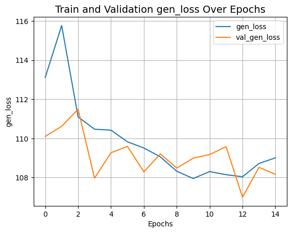
plot_history("gen_loss")
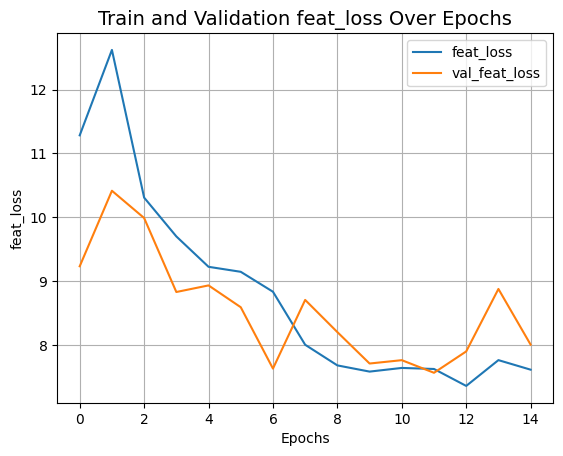
plot_history("feat_loss")
plot_history("vgg_loss")
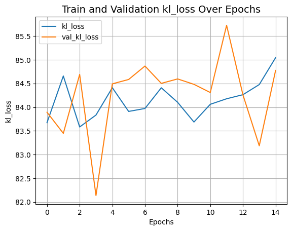
plot_history("kl_loss")
Result
Epoch 1/15

/home/sineeli/anaconda3/envs/kerasv3/lib/python3.10/site-packages/keras/src/optimizers/base_optimizer.py:472: UserWarning: Gradients do not exist for variables ['kernel', 'kernel', 'gamma', 'beta', 'kernel', 'gamma', 'beta', 'kernel', 'gamma', 'beta', 'kernel', 'gamma', 'beta', 'kernel', 'bias', 'kernel', 'bias'] when minimizing the loss. If using `model.compile()`, did you forget to provide a `loss` argument?
  warnings.warn(
WARNING: All log messages before absl::InitializeLog() is called are written to STDERR
I0000 00:00:1705013303.976306   30381 device_compiler.h:186] Compiled cluster using XLA!  This line is logged at most once for the lifetime of the process.
W0000 00:00:1705013304.021899   30381 graph_launch.cc:671] Fallback to op-by-op mode because memset node breaks graph update

 75/75 ━━━━━━━━━━━━━━━━━━━━ 0s 176ms/step - disc_loss: 1.3079 - feat_loss: 11.2902 - gen_loss: 113.0583 - kl_loss: 83.1424 - vgg_loss: 18.4966

W0000 00:00:1705013326.657730   30384 graph_launch.cc:671] Fallback to op-by-op mode because memset node breaks graph update

 1/1 ━━━━━━━━━━━━━━━━━━━━ 3s 3s/step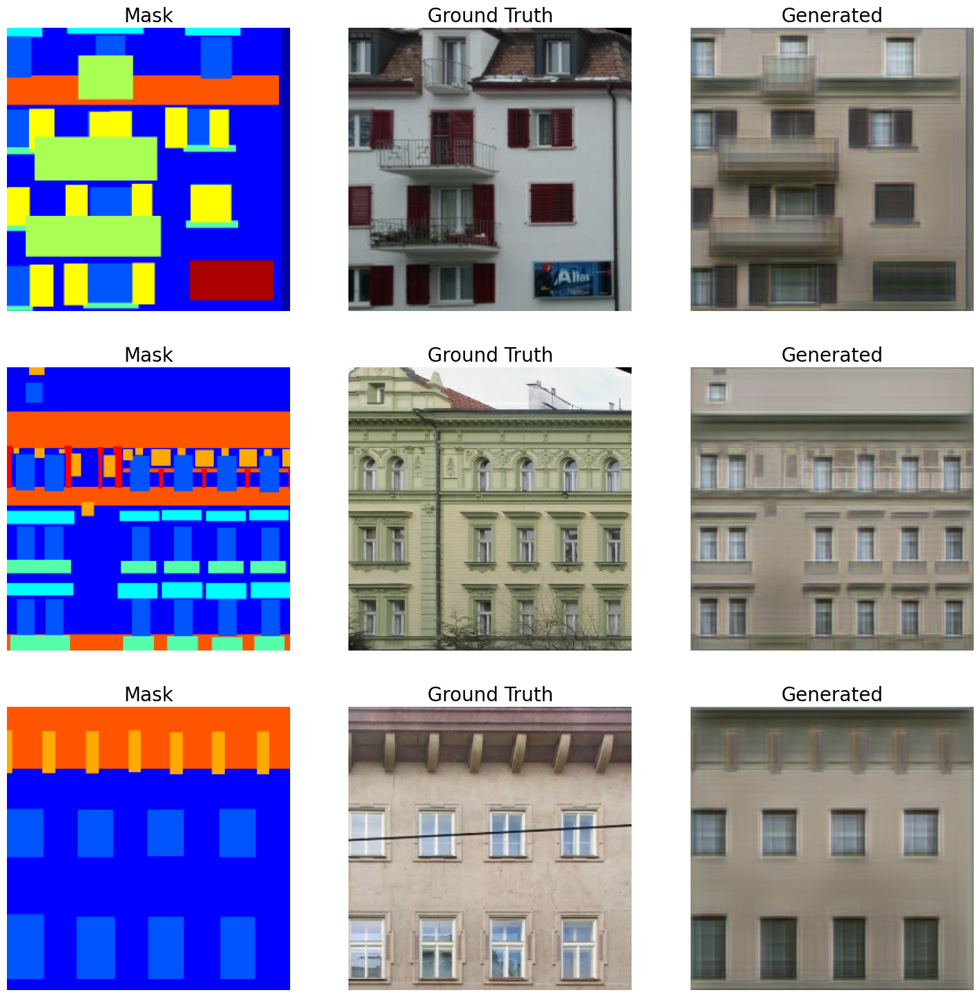


 75/75 ━━━━━━━━━━━━━━━━━━━━ 114s 426ms/step - disc_loss: 1.3051 - feat_loss: 11.2902 - gen_loss: 113.0590 - kl_loss: 83.1493 - vgg_loss: 18.4890 - val_disc_loss: 1.0374 - val_feat_loss: 9.2344 - val_gen_loss: 110.1001 - val_kl_loss: 83.8935 - val_vgg_loss: 16.6412
Epoch 2/15
 75/75 ━━━━━━━━━━━━━━━━━━━━ 14s 193ms/step - disc_loss: 0.8257 - feat_loss: 12.6603 - gen_loss: 115.9798 - kl_loss: 84.4545 - vgg_loss: 18.2973 - val_disc_loss: 0.9296 - val_feat_loss: 10.4162 - val_gen_loss: 110.6182 - val_kl_loss: 83.4473 - val_vgg_loss: 16.5499
Epoch 3/15
 75/75 ━━━━━━━━━━━━━━━━━━━━ 15s 194ms/step - disc_loss: 0.9126 - feat_loss: 10.4992 - gen_loss: 111.6962 - kl_loss: 83.8692 - vgg_loss: 17.0433 - val_disc_loss: 0.8875 - val_feat_loss: 9.9899 - val_gen_loss: 111.4879 - val_kl_loss: 84.6905 - val_vgg_loss: 16.4510
Epoch 4/15
 75/75 ━━━━━━━━━━━━━━━━━━━━ 15s 194ms/step - disc_loss: 0.8975 - feat_loss: 9.9081 - gen_loss: 111.2489 - kl_loss: 84.3098 - vgg_loss: 16.7369 - val_disc_loss: 0.9266 - val_feat_loss: 8.8318 - val_gen_loss: 107.9712 - val_kl_loss: 82.1354 - val_vgg_loss: 16.2676
Epoch 5/15
 75/75 ━━━━━━━━━━━━━━━━━━━━ 15s 194ms/step - disc_loss: 0.9378 - feat_loss: 9.1914 - gen_loss: 110.5359 - kl_loss: 84.7988 - vgg_loss: 16.3160 - val_disc_loss: 1.0073 - val_feat_loss: 8.9351 - val_gen_loss: 109.2667 - val_kl_loss: 84.4920 - val_vgg_loss: 16.3844
Epoch 6/15
 1/1 ━━━━━━━━━━━━━━━━━━━━ 0s 35ms/step


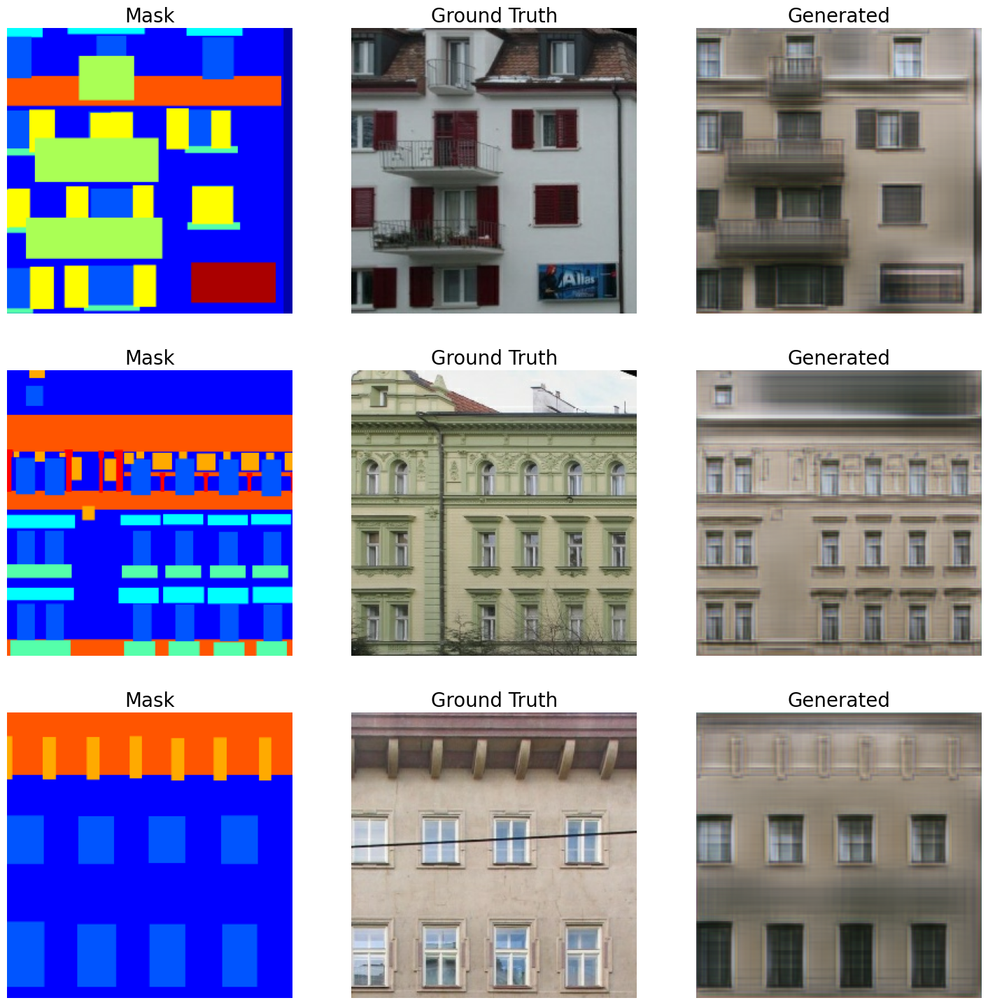
 75/75 ━━━━━━━━━━━━━━━━━━━━ 19s 258ms/step - disc_loss: 0.8982 - feat_loss: 9.2486 - gen_loss: 109.9399 - kl_loss: 83.8095 - vgg_loss: 16.5587 - val_disc_loss: 0.8061 - val_feat_loss: 8.5935 - val_gen_loss: 109.5937 - val_kl_loss: 84.5844 - val_vgg_loss: 15.8794
Epoch 7/15
 75/75 ━━━━━━━━━━━━━━━━━━━━ 15s 194ms/step - disc_loss: 0.9048 - feat_loss: 9.1064 - gen_loss: 109.3803 - kl_loss: 83.8245 - vgg_loss: 16.0975 - val_disc_loss: 1.0096 - val_feat_loss: 7.6335 - val_gen_loss: 108.2900 - val_kl_loss: 84.8679 - val_vgg_loss: 15.9580
Epoch 8/15
 75/75 ━━━━━━━━━━━━━━━━━━━━ 15s 193ms/step - disc_loss: 0.9075 - feat_loss: 8.0537 - gen_loss: 108.1771 - kl_loss: 83.6673 - vgg_loss: 16.1545 - val_disc_loss: 1.0090 - val_feat_loss: 8.7077 - val_gen_loss: 109.2079 - val_kl_loss: 84.5022 - val_vgg_loss: 16.3814
Epoch 9/15
 75/75 ━━━━━━━━━━━━━━━━━━━━ 15s 194ms/step - disc_loss: 0.9053 - feat_loss: 7.7949 - gen_loss: 107.9268 - kl_loss: 83.6504 - vgg_loss: 16.1193 - val_disc_loss: 1.0663 - val_feat_loss: 8.2042 - val_gen_loss: 108.4819 - val_kl_loss: 84.5961 - val_vgg_loss: 16.0834
Epoch 10/15
 75/75 ━━━━━━━━━━━━━━━━━━━━ 15s 194ms/step - disc_loss: 0.8905 - feat_loss: 7.7652 - gen_loss: 108.3079 - kl_loss: 83.8574 - vgg_loss: 16.2992 - val_disc_loss: 0.8362 - val_feat_loss: 7.7127 - val_gen_loss: 108.9906 - val_kl_loss: 84.4822 - val_vgg_loss: 16.0521
Epoch 11/15
 1/1 ━━━━━━━━━━━━━━━━━━━━ 0s 30ms/step


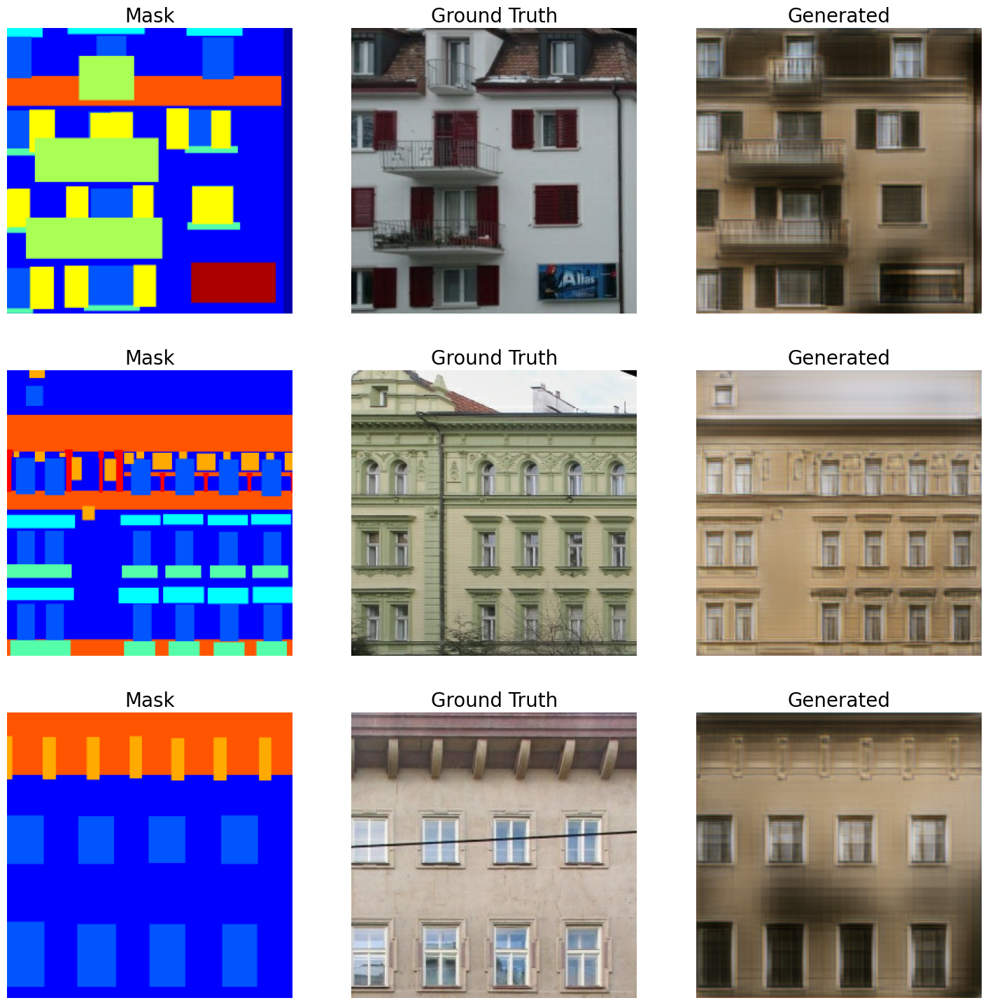
 75/75 ━━━━━━━━━━━━━━━━━━━━ 20s 263ms/step - disc_loss: 0.9047 - feat_loss: 7.5019 - gen_loss: 107.6317 - kl_loss: 83.6812 - vgg_loss: 16.1292 - val_disc_loss: 0.8788 - val_feat_loss: 7.7651 - val_gen_loss: 109.1731 - val_kl_loss: 84.3094 - val_vgg_loss: 16.0356
Epoch 12/15
 75/75 ━━━━━━━━━━━━━━━━━━━━ 15s 194ms/step - disc_loss: 0.8899 - feat_loss: 7.5799 - gen_loss: 108.2313 - kl_loss: 84.4031 - vgg_loss: 15.9665 - val_disc_loss: 0.8358 - val_feat_loss: 7.5676 - val_gen_loss: 109.5789 - val_kl_loss: 85.7282 - val_vgg_loss: 16.0442
Epoch 13/15
 75/75 ━━━━━━━━━━━━━━━━━━━━ 15s 194ms/step - disc_loss: 0.8542 - feat_loss: 7.3362 - gen_loss: 107.4649 - kl_loss: 83.6942 - vgg_loss: 16.0675 - val_disc_loss: 1.0853 - val_feat_loss: 7.9020 - val_gen_loss: 106.9958 - val_kl_loss: 84.2610 - val_vgg_loss: 15.8510
Epoch 14/15
 75/75 ━━━━━━━━━━━━━━━━━━━━ 15s 194ms/step - disc_loss: 0.8631 - feat_loss: 7.6403 - gen_loss: 108.6401 - kl_loss: 84.5304 - vgg_loss: 16.0426 - val_disc_loss: 0.9516 - val_feat_loss: 8.8795 - val_gen_loss: 108.5215 - val_kl_loss: 83.1849 - val_vgg_loss: 16.3289
Epoch 15/15
 75/75 ━━━━━━━━━━━━━━━━━━━━ 15s 194ms/step - disc_loss: 0.8939 - feat_loss: 7.5489 - gen_loss: 108.8330 - kl_loss: 85.0358 - vgg_loss: 15.9147 - val_disc_loss: 0.9616 - val_feat_loss: 8.0080 - val_gen_loss: 108.1650 - val_kl_loss: 84.7754 - val_vgg_loss: 15.9561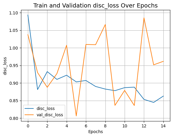

Inference
val_iterator = iter(val_dataset)

for _ in range(5):
    val_images = next(val_iterator)
    # Sample latent from a normal distribution.
    latent_vector = keras.random.normal(
        shape=(gaugan.batch_size, gaugan.latent_dim), mean=0.0, stddev=2.0
    )
    # Generate fake images.
    fake_images = gaugan.predict([latent_vector, val_images[2]])

    real_images = val_images
    grid_row = min(fake_images.shape[0], 3)
    grid_col = 3
    f, axarr = plt.subplots(grid_row, grid_col, figsize=(grid_col * 6, grid_row * 6))
    for row in range(grid_row):
        ax = axarr if grid_row == 1 else axarr[row]
        ax[0].imshow((real_images[0][row] + 1) / 2)
        ax[0].axis("off")
        ax[0].set_title("Mask", fontsize=20)
        ax[1].imshow((real_images[1][row] + 1) / 2)
        ax[1].axis("off")
        ax[1].set_title("Ground Truth", fontsize=20)
        ax[2].imshow((fake_images[row] + 1) / 2)
        ax[2].axis("off")
        ax[2].set_title("Generated", fontsize=20)
    plt.show()
Result
1/1 ━━━━━━━━━━━━━━━━━━━━ 0s 29ms/step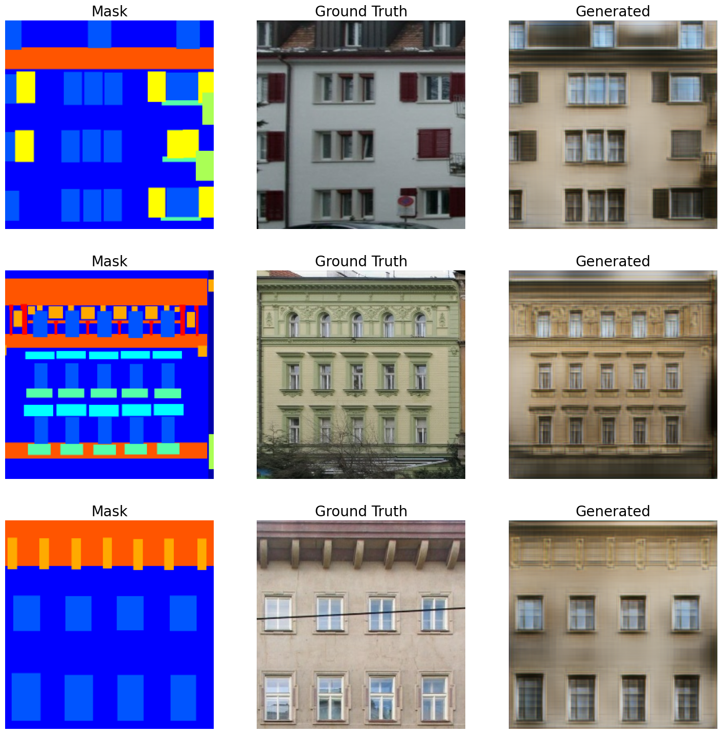
1/1 ━━━━━━━━━━━━━━━━━━━━ 0s 25ms/step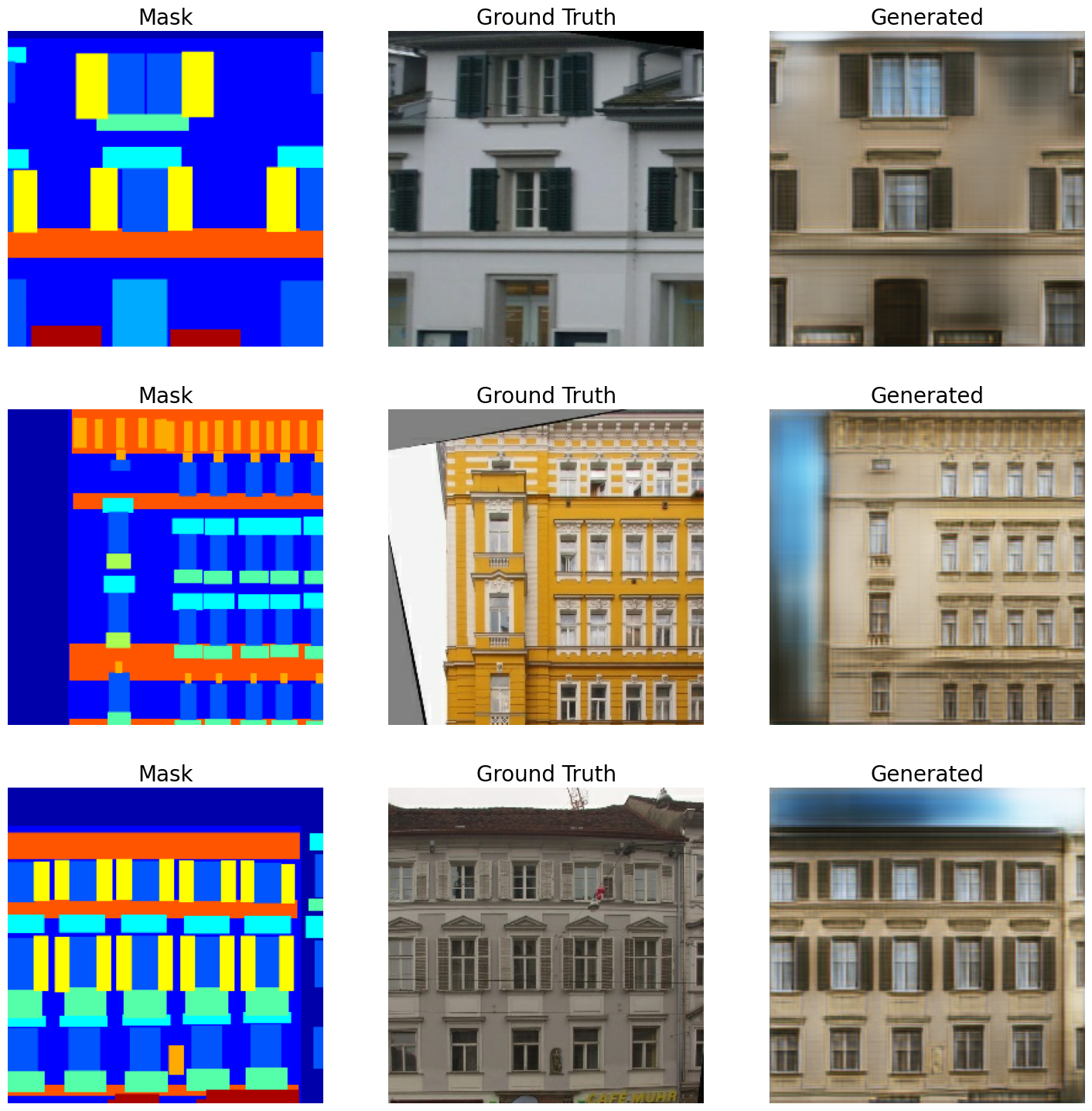
1/1 ━━━━━━━━━━━━━━━━━━━━ 0s 25ms/step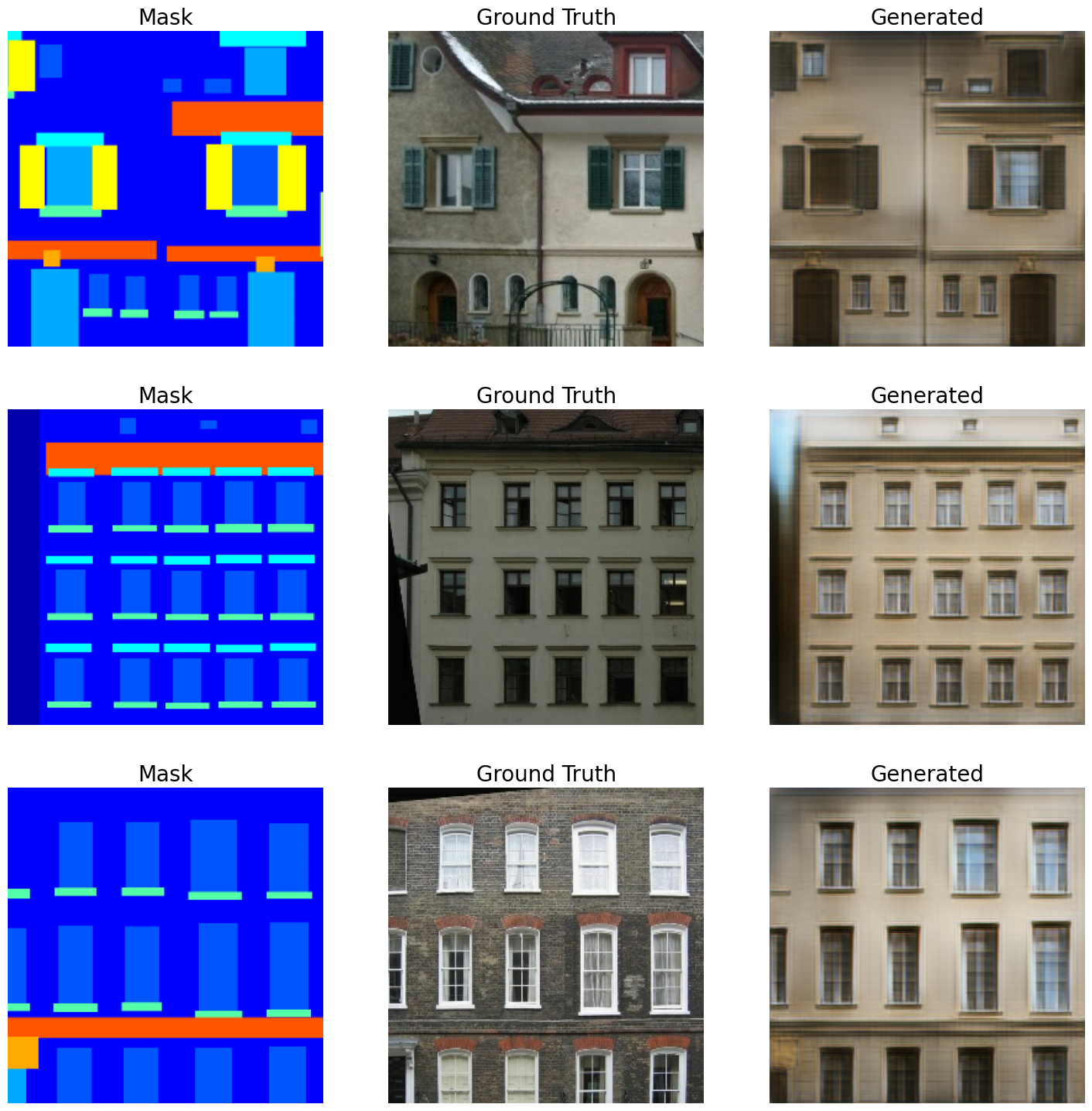
Final words
- The dataset we used in this example is a small one. For obtaining even better results we recommend to use a bigger dataset. GauGAN results were demonstrated with the COCO-Stuff and CityScapes datasets.
- This example was inspired the Chapter 6 of Hands-On Image Generation with TensorFlow by Soon-Yau Cheong and Implementing SPADE using fastai by Divyansh Jha.
- If you found this example interesting and exciting, you might want to check out our repository which we are currently building. It will include reimplementations of popular GANs and pretrained models. Our focus will be on readability and making the code as accessible as possible. Our plain is to first train our implementation of GauGAN (following the code of this example) on a bigger dataset and then make the repository public. We welcome contributions!
- Recently GauGAN2 was also released. You can check it out here.
Example available on HuggingFace.
| Trained Model | Demo |
|---|---|
 |  |